De Boor's algorithm

In the mathematical subfield of numerical analysis, de Boor's algorithm^[1] is a polynomial-time and numerically stablealgorithm for evaluating spline curves in B-spline form. It is a generalization of de Casteljau's algorithm for Bézier curves. The algorithm was devised by German-American mathematician Carl R. de Boor. Simplified, potentially faster variants of the de Boor algorithm have been created but they suffer from comparatively lower stability.^[2][3]

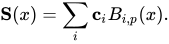
A general introduction to B-splines is given in the main article. Here we discuss de Boor's algorithm, an efficient and numerically stable scheme to evaluate a spline curve ${\displaystyle \mathbf {S} (x)}$ at position ${\displaystyle x}$. The curve is built from a sum of B-spline functions ${\displaystyle B_{i,p}(x)}$ multiplied with potentially vector-valued constants ${\displaystyle \mathbf {c} _{i}}$, called control points, $${\displaystyle \mathbf {S} (x)=\sum _{i}\mathbf {c} _{i}B_{i,p}(x).}$$ B-splines of order ${\displaystyle p+1}$ are connected piece-wise polynomial functions of degree ${\displaystyle p}$ defined over a grid of knots ${\displaystyle {t_{0},\dots ,t_{i},\dots ,t_{m}}}$ (we always use zero-based indices in the following). De Boor's algorithm uses O(p²) + O(p) operations to evaluate the spline curve. Note: the main article about B-splines and the classic publications^[1] use a different notation: the B-spline is indexed as ${\displaystyle B_{i,n}(x)}$ with ${\displaystyle n=p+1}$.

B-splines have local support, meaning that the polynomials are positive only in a compact domain and zero elsewhere. The Cox-de Boor recursion formula^[4] shows this: $${\displaystyle B_{i,0}(x):={\begin{cases}1&{\text{if }}\quad t_{i}\leq x<t_{i+1}\\0&{\text{otherwise}}\end{cases}}}$$$${\displaystyle B_{i,p}(x):={\frac {x-t_{i}}{t_{i+p}-t_{i}}}B_{i,p-1}(x)+{\frac {t_{i+p+1}-x}{t_{i+p+1}-t_{i+1}}}B_{i+1,p-1}(x).}$$

Let the index ${\displaystyle k}$ define the knot interval that contains the position, ${\displaystyle x\in [t_{k},t_{k+1})}$. We can see in the recursion formula that only B-splines with ${\displaystyle i=k-p,\dots ,k}$ are non-zero for this knot interval. Thus, the sum is reduced to: $${\displaystyle \mathbf {S} (x)=\sum _{i=k-p}^{k}\mathbf {c} _{i}B_{i,p}(x).}$$

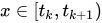
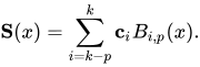
It follows from ${\displaystyle i\geq 0}$ that ${\displaystyle k\geq p}$. Similarly, we see in the recursion that the highest queried knot location is at index ${\displaystyle k+1+p}$. This means that any knot interval ${\displaystyle [t_{k},t_{k+1})}$ which is actually used must have at least ${\displaystyle p}$ additional knots before and after. In a computer program, this is typically achieved by repeating the first and last used knot location ${\displaystyle p}$ times. For example, for ${\displaystyle p=3}$ and real knot locations ${\displaystyle (0,1,2)}$, one would pad the knot vector to ${\displaystyle (0,0,0,0,1,2,2,2,2)}$.

With these definitions, we can now describe de Boor's algorithm. The algorithm does not compute the B-spline functions ${\displaystyle B_{i,p}(x)}$ directly. Instead it evaluates ${\displaystyle \mathbf {S} (x)}$ through an equivalent recursion formula.

Let ${\displaystyle \mathbf {d} _{i,r}}$ be new control points with ${\displaystyle \mathbf {d} _{i,0}:=\mathbf {c} _{i}}$ for ${\displaystyle i=k-p,\dots ,k}$. For ${\displaystyle r=1,\dots ,p}$ the following recursion is applied: $${\displaystyle \mathbf {d} _{i,r}=(1-\alpha _{i,r})\mathbf {d} _{i-1,r-1}+\alpha _{i,r}\mathbf {d} _{i,r-1};\quad i=k-p+r,\dots ,k}$$$${\displaystyle \alpha _{i,r}={\frac {x-t_{i}}{t_{i+1+p-r}-t_{i}}}.}$$

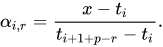
Once the iterations are complete, we have ${\displaystyle \mathbf {S} (x)=\mathbf {d} _{k,p}}$, meaning that ${\displaystyle \mathbf {d} _{k,p}}$ is the desired result.

De Boor's algorithm is more efficient than an explicit calculation of B-splines ${\displaystyle B_{i,p}(x)}$ with the Cox-de Boor recursion formula, because it does not compute terms which are guaranteed to be multiplied by zero.

The algorithm above is not optimized for the implementation in a computer. It requires memory for ${\displaystyle (p+1)+p+\dots +1=(p+1)(p+2)/2}$ temporary control points ${\displaystyle \mathbf {d} _{i,r}}$. Each temporary control point is written exactly once and read twice. By reversing the iteration over ${\displaystyle i}$ (counting down instead of up), we can run the algorithm with memory for only ${\displaystyle p+1}$ temporary control points, by letting ${\displaystyle \mathbf {d} _{i,r}}$ reuse the memory for ${\displaystyle \mathbf {d} _{i,r-1}}$. Similarly, there is only one value of ${\displaystyle \alpha }$ used in each step, so we can reuse the memory as well.

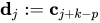
Furthermore, it is more convenient to use a zero-based index ${\displaystyle j=0,\dots ,p}$ for the temporary control points. The relation to the previous index is ${\displaystyle i=j+k-p}$. Thus we obtain the improved algorithm:

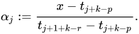
Let ${\displaystyle \mathbf {d} _{j}:=\mathbf {c} _{j+k-p}}$ for ${\displaystyle j=0,\dots ,p}$. Iterate for ${\displaystyle r=1,\dots ,p}$: $${\displaystyle \mathbf {d} _{j}:=(1-\alpha _{j})\mathbf {d} _{j-1}+\alpha _{j}\mathbf {d} _{j};\quad j=p,\dots ,r\quad }$$$${\displaystyle \alpha _{j}:={\frac {x-t_{j+k-p}}{t_{j+1+k-r}-t_{j+k-p}}}.}$$ Note that j must be counted down. After the iterations are complete, the result is ${\displaystyle \mathbf {S} (x)=\mathbf {d} _{p}}$.

The following code in the Python programming language is a naive implementation of the optimized algorithm.

defdeBoor(k:int,x:int,t,c,p:int):"""Evaluates S(x). Arguments --------- k: Index of knot interval that contains x. x: Position. t: Array of knot positions, needs to be padded as described above. c: Array of control points. p: Degree of B-spline. """d=[c[j+k-p]forjinrange(0,p+1)]forrinrange(1,p+1):forjinrange(p,r-1,-1):alpha=(x-t[j+k-p])/(t[j+1+k-r]-t[j+k-p])d[j]=(1.0-alpha)*d[j-1]+alpha*d[j]returnd[p]

• De Casteljau's algorithm
• Bézier curve
• Non-uniform rational B-spline

• De Boor's Algorithm
• The DeBoor-Cox Calculation

• PPPACK: contains many spline algorithms in Fortran
• GNU Scientific Library: C-library, contains a sub-library for splines ported from PPPACK
• SciPy: Python-library, contains a sub-library scipy.interpolate with spline functions based on FITPACK
• TinySpline: C-library for splines with a C++ wrapper and bindings for C#, Java, Lua, PHP, Python, and Ruby
• Einspline: C-library for splines in 1, 2, and 3 dimensions with Fortran wrappers

Works cited

• Carl de Boor (2003). A Practical Guide to Splines, Revised Edition. Springer-Verlag. ISBN 0-387-95366-3.

References

- 12C. de Boor [1971], "Subroutine package for calculating with B-splines", Techn.Rep. LA-4728-MS, Los Alamos Sci.Lab, Los Alamos NM; p. 109, 121.
- ↑Lee, E. T. Y. (December 1982). "A Simplified B-Spline Computation Routine". Computing. 29 (4). Springer-Verlag: 365–371. doi:10.1007/BF02246763. S2CID 2407104.
- ↑Lee, E. T. Y. (1986). "Comments on some B-spline algorithms". Computing. 36 (3). Springer-Verlag: 229–238. doi:10.1007/BF02240069. S2CID 7003455.