Central composite design

In statistics, a central composite design is an experimental design, useful in response surface methodology, for building a second order (quadratic) model for the response variable without needing to use a complete three-level factorial experiment.

After the designed experiment is performed, linear regression is used, sometimes iteratively, to obtain results. Coded variables are often used when constructing this design.

The design consists of three distinct sets of experimental runs:

1. A factorial (perhaps fractional) design in the factors studied, each having two levels;
2. A set of center points, experimental runs whose values of each factor are the medians of the values used in the factorial portion. This point is often replicated in order to improve the precision of the experiment;
3. A set of axial points, experimental runs identical to the centre points except for one factor, which will take on values both below and above the median of the two factorial levels, and typically both outside their range. All factors are varied in this way.

The design matrix for a central composite design experiment involving k factors is derived from a matrix, d, containing the following three different parts corresponding to the three types of experimental runs:

1. The matrix F obtained from the factorial experiment. The factor levels are scaled so that its entries are coded as +1 and −1.
2. The matrix C from the center points, denoted in coded variables as (0,0,0,...,0), where there are k zeros.
3. A matrix E from the axial points, with 2k rows. Each factor is sequentially placed at ±α and all other factors are at zero. The value of α is determined by the designer; while arbitrary, some values may give the design desirable properties. This part would look like:

${\displaystyle \mathbf {E} ={\begin{bmatrix}\alpha &0&0&\cdots &\cdots &\cdots &0\\{-\alpha }&0&0&\cdots &\cdots &\cdots &0\\0&\alpha &0&\cdots &\cdots &\cdots &0\\0&{-\alpha }&0&\cdots &\cdots &\cdots &0\\\vdots &{}&{}&{}&{}&{}&\vdots \\0&0&0&0&\cdots &\cdots &\alpha \\0&0&0&0&\cdots &\cdots &{-\alpha }\\\end{bmatrix}}.}$

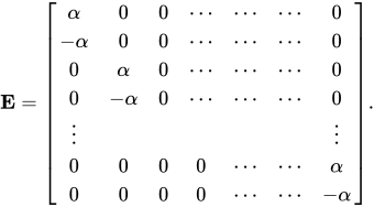
Then d is the vertical concatenation:

${\displaystyle \mathbf {d} ={\begin{bmatrix}\mathbf {F} \\\mathbf {C} \\\mathbf {E} \end{bmatrix}}.}$

The design matrix X used in linear regression is the horizontal concatenation of a column of 1s (intercept), d, and all elementwise products of a pair of columns of d:

${\displaystyle \mathbf {X} ={\begin{bmatrix}\mathbf {1} &\mathbf {d} &\mathbf {d} (1)\times \mathbf {d} (2)&\mathbf {d} (1)\times \mathbf {d} (3)&\cdots &\mathbf {d} (k-1)\times \mathbf {d} (ك)&\mathbf {d} (1)^{2}&\mathbf {d} (2)^{2}&\cdots &\mathbf {d} (k)^{2}\end{bmatrix}},}$

where d(i) represents the ith column in d.

مايرز، ريموند هـ. منهجية سطح الاستجابة . بوسطن: ألين وبيكون، 1971