
Plane stress
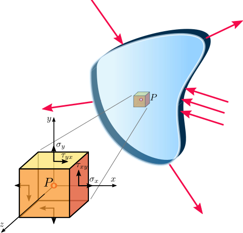
In continuum mechanics, a material is said to be under plane stress if the stress vector is zero across a particular plane. When that situation occurs over an entire element of a structure, as is often the case for thin plates, the stress analysis is considerably simplified, as the stress state can be represented by a tensor of dimension 2 (representable as a 2×2 matrix rather than 3×3). [1] A related notion, plane strain, is often applicable to very thick members.
Plane stress typically occurs in thin flat plates that are acted upon only by load forces that are parallel to them. In certain situations, a gently curved thin plate may also be assumed to have plane stress for the purpose of stress analysis. This is the case, for example, of a thin-walled cylinder filled with a fluid under pressure. In such cases, stress components perpendicular to the plate are negligible compared to those parallel to it.[1]
In other situations, however, the bending stress of a thin plate cannot be neglected. One can still simplify the analysis by using a two-dimensional domain, but the plane stress tensor at each point must be complemented with bending terms.
Mathematical definition
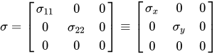
Mathematically, the stress at some point in the material is a plane stress if one of the three principal stresses (the eigenvalues of the Cauchy stress tensor) is zero. That is, there is Cartesian coordinate system in which the stress tensor has the form
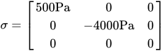
For example, consider a rectangular block of material measuring 10, 40 and 5 cm along the , , and , that is being stretched in the direction and compressed in the direction, by pairs of opposite forces with magnitudes 10 N and 20 N, respectively, uniformly distributed over the corresponding faces. The stress tensor inside the block will be


More generally, if one chooses the first two coordinate axes arbitrarily but perpendicular to the direction of zero stress, the stress tensor will have the form
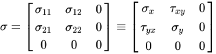
and can therefore be represented by a 2 × 2 matrix,
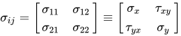
Constitutive equations
Plane stress in curved surfaces
في بعض الحالات، يمكن استخدام نموذج الإجهاد المستوي في تحليل الأسطح المنحنية انحناءً طفيفًا. على سبيل المثال، لنفترض أسطوانة رقيقة الجدران تتعرض لحمل ضغط محوري موزع بانتظام على طول حافتها، ومملوءة بسائل مضغوط. سيولد الضغط الداخلي إجهادًا حلقيًا تفاعليًا على الجدار، وإجهاد شد عموديًا موجهًا بشكل عمودي على محور الأسطوانة ومماسًا لسطحها. يمكن اعتبار الأسطوانة، من الناحية النظرية، صفيحة مستطيلة رقيقة مسطحة تتعرض لحمل شد في اتجاه وحمل ضغط في اتجاه آخر، وكلاهما موازٍ للصفيحة.
الإجهاد المستوي (مصفوفة الإجهاد)
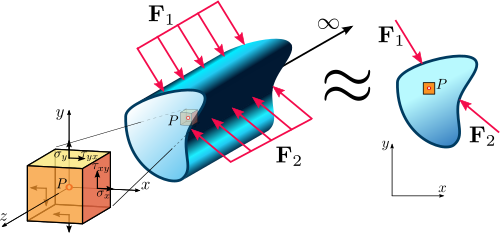
إذا كان أحد الأبعاد كبيرًا جدًا مقارنةً بالأبعاد الأخرى، فإن الإجهاد الرئيسي في اتجاه أطول بُعد يكون محدودًا ويمكن افتراض ثباته، مما يعني انعدام الإجهاد فعليًا على طوله، وبالتالي الحصول على حالة إجهاد مستوٍ (الشكل 7.2). في هذه الحالة، على الرغم من أن جميع الإجهادات الرئيسية لا تساوي صفرًا، إلا أنه يمكن إهمال الإجهاد الرئيسي في اتجاه أطول بُعد في الحسابات. وهذا يسمح بإجراء تحليل ثنائي الأبعاد للإجهادات، على سبيل المثال ، تحليل سد عند مقطع عرضي مُحمّل بالخزان.
موتر الإجهاد المقابل هو:
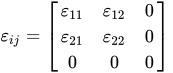
وموتر الإجهاد المقابل هو:
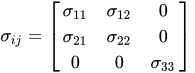
حيث غير الصفرينشأ هذا الحد من تأثير بواسون . ومع ذلك، يمكن إزالة هذا الحد مؤقتًا من تحليل الإجهاد بحيث لا يتبقى سوى الحدود الموجودة في المستوى، مما يقلل التحليل فعليًا إلى بعدين. [ 1 ]

تحول الإجهاد في الإجهاد المستوي والانفعال المستوي
لنفترض نقطةفي وسط متصل تحت حالة إجهاد مستوٍ، أو انفعال مستوٍ، مع مكونات الإجهادوجميع مكونات الإجهاد الأخرى تساوي صفرًا (الشكل 8.1). من التوازن الساكن لعنصر مادي متناهي الصغر عند(الشكل 8.2)، الإجهاد الطبيعيوإجهاد القصعلى أي مستوى عمودي على-طائرة تمر عبربمتجه وحدةصنع زاوية منمع الأفقي، أيهو جيب تمام الاتجاه فييتم تحديد الاتجاه بواسطة:



تشير هذه المعادلات إلى أنه في حالة الإجهاد المستوي أو الانفعال المستوي، يمكن تحديد مركبات الإجهاد عند نقطة ما في جميع الاتجاهات، أي كدالة لـإذا كان المرء على دراية بمكونات الإجهادعلى أي اتجاهين متعامدين عند تلك النقطة. من المهم أن نتذكر أننا نأخذ في الاعتبار وحدة مساحة العنصر المتناهي الصغر في الاتجاه الموازي لـ-طائرة.

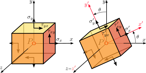

يمكن الحصول على الاتجاهات الرئيسية (الشكل 8.3)، أي اتجاه المستويات التي تكون فيها مركبات إجهاد القص صفرًا، من خلال تطبيق المعادلة السابقة لإجهاد القص.يساوي صفرًا. وبالتالي لدينا:

ونحصل
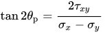
تحدد هذه المعادلة قيمتينوهيمتباعدين (الشكل 8.3). ويمكن الحصول على النتيجة نفسها بإيجاد الزاويةمما يجعل الإجهاد طبيعياًالحد الأقصى، أي


يؤكد المديروأو الحد الأدنى والحد الأقصى للإجهادات الطبيعيةوويمكن الحصول على القيمتين، على التوالي، عن طريق استبدال كلتا القيمتين بـفي المعادلة السابقة لـويمكن تحقيق ذلك عن طريق إعادة ترتيب المعادلات لـوأولاً، نقوم بنقل الحد الأول في المعادلة الأولى، ثم نربع طرفي كل معادلة، ثم نجمعهما. وهكذا نحصل على


![{\displaystyle \left[\sigma _{\mathrm {n} }-{\tfrac {1}{2}}(\sigma _{x}+\sigma _{y})\right]^{2}+\tau _{\mathrm {n} }^{2}=\left[{\tfrac {1}{2}}(\sigma _{x}-\sigma _{y})\right]^{2}+\tau _{xy}^{2}\,\!}](https://wikimedia.org/api/rest_v1/media/math/render/svg/6663836ffd3a152f45b88c231803e9b87b847e4d)

أين
![{\displaystyle R={\sqrt {\left[{\tfrac {1}{2}}(\sigma _{x}-\sigma _{y})\right]^{2}+\tau _{xy}^{2}}}\quad {\text{and}}\quad \sigma _{\mathrm {avg} }={\tfrac {1}{2}}(\sigma _{x}+\sigma _{y})\,\!}](https://wikimedia.org/api/rest_v1/media/math/render/svg/d51778d2496ae782c15426280a6a962558be0945)
وهي معادلة دائرة نصف قطرهامتمركزة عند نقطة ذات إحداثياتتُسمى دائرة مور . ولكن مع العلم أن الإجهادات الرئيسية هي إجهاد القصومن ثم نحصل من هذه المعادلة على ما يلي:

![{\displaystyle [\sigma _{\mathrm {avg} },0]\,\!}](https://wikimedia.org/api/rest_v1/media/math/render/svg/0927454621022374baf886469fd3f01c7f3aa074)

![{\displaystyle \sigma _{1}=\sigma _{\mathrm {max} }={\tfrac {1}{2}}(\sigma _{x}+\sigma _{y})+{\sqrt {\left[{\tfrac {1}{2}}(\sigma _{x}-\sigma _{y})\right]^{2}+\tau _{xy}^{2}}}\,\!}](https://wikimedia.org/api/rest_v1/media/math/render/svg/b5a9ef37e9ce22a5af1bb69f44e4fc8122e0f0a2)
![{\displaystyle \sigma _{2}=\sigma _{\mathrm {min} }={\tfrac {1}{2}}(\sigma _{x}+\sigma _{y})-{\sqrt {\left[{\tfrac {1}{2}}(\sigma _{x}-\sigma _{y})\right]^{2}+\tau _{xy}^{2}}}\,\!}](https://wikimedia.org/api/rest_v1/media/math/render/svg/7e28c9ab361ed0a4fb553d9840db1c8fc0a88dd6)
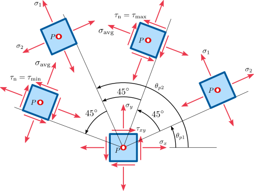
متىيتم توجيه العنصر المتناهي الصغر في اتجاه المستويات الرئيسية، وبالتالي فإن الإجهادات المؤثرة على العنصر المستطيل هي إجهادات رئيسية:وثم الإجهاد الطبيعيوإجهاد القصيمكن تحديدها كدالة للإجهادات الرئيسية عن طريق جعلوهكذا لدينا



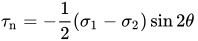
ثم أقصى إجهاد قصيحدث ذلك عندما ، أي(الشكل 8.3):


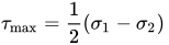
ثم الحد الأدنى لإجهاد القصيحدث ذلك عندما ، أي(الشكل 8.3):


انظر أيضاً
مراجع
- علم المعادن
- الهندسة الميكانيكية