
توزيع الجيب العكسي
في نظرية الاحتمالات ، يُعد توزيع الجيب العكسي هو توزيع الاحتمالات الذي تتضمن دالة التوزيع التراكمي الخاصة به الجيب العكسي والجذر التربيعي :

لـ 0 ≤ x ≤ 1، ودالة كثافة الاحتمال الخاصة بها هي
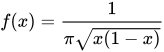
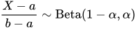
على الفترة (0، 1). يُعد توزيع الجيب العكسي القياسي حالة خاصة من توزيع بيتا حيث α = β = 1/2. أي، إذا إذا كان متغيرًا عشوائيًا يتبع توزيع الجيب العكسي،وبالتالي، فإن توزيع الجيب العكسي هو حالة خاصة من توزيع بيرسون من النوع الأول .

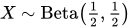
يظهر توزيع دالة الجيب العكسي في قانون ليفي لدالة الجيب العكسي ، وفي قانون إردوش لدالة الجيب العكسي ، وكتوزيع جيفريز المسبق لاحتمالية نجاح تجربة برنولي . [ 1 ] [ 2 ] كثافة احتمال دالة الجيب العكسي هي توزيع يظهر في العديد من النظريات الأساسية للمشي العشوائي. في المشي العشوائي لرمية عملة عادلة ، يتوزع احتمال وقت آخر زيارة إلى نقطة الأصل كتوزيع دالة الجيب العكسي (على شكل حرف U) . [ 3 ] [ 4 ] في لعبة رمي عملة عادلة بين لاعبين، يُقال إن اللاعب متقدم إذا كان مساره العشوائي (الذي بدأ من نقطة الأصل) أعلى من نقطة الأصل. إن العدد الأكثر احتمالاً لعدد المرات التي يكون فيها لاعب معين متقدمًا، في لعبة طولها 2N ، ليس N. على العكس من ذلك، فإن N هو العدد الأقل احتمالاً لعدد المرات التي يكون فيها اللاعب متقدمًا. عدد المرات الأكثر احتمالاً للتقدم هو 0 أو 2 N (وفقًا لتوزيع دالة الجيب العكسي).
تعميم
دعم محدود عشوائي
يمكن توسيع التوزيع ليشمل أي نطاق محدود من a ≤ x ≤ b عن طريق تحويل بسيط
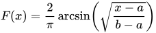
لـ a ≤ x ≤ b ، ودالة كثافة الاحتمال الخاصة بها هي
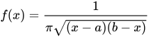
على ( أ ، ب ).
عامل الشكل
توزيع الجيب العكسي القياسي المعمم على الفترة (0،1) بدالة كثافة احتمالية

وهي أيضاً حالة خاصة من توزيع بيتا ذي المعاملات.

لاحظ أنه عندمايختزل توزيع الجيب العكسي العام إلى التوزيع القياسي المذكور أعلاه.

ملكيات
- توزيع دالة الجيب العكسي مغلق تحت الإزاحة والقياس بمعامل موجب
- لو
- The square of an arcsine distribution over (-1, 1) has arcsine distribution over (0, 1)
- If
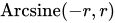
- The coordinates of points uniformly selected on a circle of radius centered at the origin (0, 0), have an distribution
- For example, if we select a point uniformly on the circumference, , we have that the point's x coordinate distribution is , and its y coordinate distribution is






Characteristic function
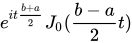
The characteristic function of the generalized arcsine distribution is a zero order Bessel function of the first kind, multiplied by a complex exponential, given by . For the special case of , the characteristic function takes the form of .


Related distributions





References
- ↑Overturf, Drew; et al. (2017). Investigation of beamforming patterns from volumetrically distributed phased arrays. MILCOM 2017 - 2017 IEEE Military Communications Conference (MILCOM). pp. 817–822. doi:10.1109/MILCOM.2017.8170756. ISBN 978-1-5386-0595-0.
- ↑Buchanan, K.; et al. (2020). "Null Beamsteering Using Distributed Arrays and Shared Aperture Distributions". IEEE Transactions on Antennas and Propagation. 68 (7): 5353–5364. Bibcode:2020ITAP...68.5353B. doi:10.1109/TAP.2020.2978887.
- ↑Feller, William (1971). An Introduction to Probability Theory and Its Applications, Vol. 2. Wiley. ISBN 978-0471257097.
- ↑Feller, William (1968). An Introduction to Probability Theory and Its Applications. Vol. 1 (3rd ed.). Wiley. ISBN 978-0471257080.
Further reading
- Rogozin, B.A. (2001) [1994], "Arcsine distribution", Encyclopedia of Mathematics, EMS Press
- Continuous distributions