
توزيع بيتا
في نظرية الاحتمالات والإحصاء ، فإن توزيع بيتا هو عائلة من توزيعات الاحتمالات المستمرة المعرفة على الفترة [0، 1] أو (0، 1) من حيث معلمتين موجبتين ، يرمز لهما بـ ألفا ( α ) وبيتا ( β ) ، واللتان تظهران كأسين للمتغير ومكمله لـ 1، على التوالي، وتتحكمان في شكل التوزيع.
تم تطبيق توزيع بيتا لنمذجة سلوك المتغيرات العشوائية المقتصرة على فترات ذات طول محدود في العديد من التخصصات. ويُعد توزيع بيتا نموذجًا مناسبًا للسلوك العشوائي للنسب المئوية والنسب.
في الاستدلال البايزي ، يعتبر توزيع بيتا هو التوزيع الاحتمالي المسبق المترافق لتوزيعات برنولي ، وذو الحدين ، وذو الحدين السالب ، والهندسي .
يُعرف نموذج توزيع بيتا المذكور هنا أيضًا باسم توزيع بيتا من النوع الأول ، بينما يُعد توزيع بيتا من النوع الثاني اسمًا بديلًا لتوزيع بيتا الأولي . ويُطلق على التعميم ليشمل متغيرات متعددة اسم توزيع ديريشليه .
التعريفات
دالة كثافة الاحتمال

دالة كثافة الاحتمال (PDF) لتوزيع بيتا، لـأو، ومعاملات الشكل،، هي دالة أسية للمتغيروانعكاسهاعلى النحو التالي:


![{\displaystyle {\begin{aligned}f(x;\alpha ,\beta )&=\mathrm {constant} \cdot x^{\alpha -1}(1-x)^{\beta -1}\\[3pt]&={\frac {x^{\alpha -1}(1-x)^{\beta -1}}{\displaystyle \int _ {0}^{1}u^{\alpha -1}(1-u)^{\beta -1}\,du}}\\[6pt]&={\frac {\Gamma (\alpha +\beta )}{\Gamma (\alpha )\Gamma (\beta )}}\,x^{\alpha -1}(1-x)^{\beta -1}\\[6pt]&={\frac {1}{\mathrm {B} (\alpha ,\beta )}}x^{\alpha -1}(1-x)^{\beta -1}\end{aligned}}}](https://wikimedia.org/api/rest_v1/media/math/render/svg/5fc18388353b219c482e8e35ca4aae808ab1be81)
أيندالة غاما . دالة بيتا ،، هو ثابت توحيد لضمان أن يكون الاحتمال الكلي 1. في المعادلات أعلاههو تحقق - قيمة مُلاحظة حدثت بالفعل - لمتغير عشوائي.


يستخدم العديد من المؤلفين، بمن فيهم إن إل جونسون وإس كوتز ، [ 1 ] الرموزو(بدلاً منو) بالنسبة لمعاملات شكل توزيع بيتا، والتي تُذكّر بالرموز المستخدمة تقليديًا لمعاملات توزيع برنولي ، لأن توزيع بيتا يقترب من توزيع برنولي في حالة الحد عندما تكون كلتا معاملتي الشكلوالاقتراب من الصفر.


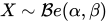
فيما يلي، متغير عشوائيموزع بيتا مع معلماتوسيتم الإشارة إليها بـ: [ 2 ] [ 3 ]

تتضمن الرموز الأخرى المستخدمة في الأدبيات الإحصائية للمتغيرات العشوائية ذات التوزيع بيتا ما يلي:[ 4 ] و[ 5 ]

دالة التوزيع التراكمي


دالة التوزيع التراكمي هي

أينهي دالة بيتا غير المكتملة وهي دالة بيتا غير الكاملة المنتظمة .


بالنسبة للأعداد الصحيحة الموجبة α و β ، يمكن التعبير عن دالة التوزيع التراكمي لتوزيع بيتا بدلالة دالة التوزيع التراكمي لتوزيع ذي الحدين مع [ 6 ]

المعلمات البديلة
معياران
المتوسط وحجم العينة
يمكن إعادة تمثيل توزيع بيتا بدلالة متوسطه μ (0 < μ < 1) ومجموع معاملي الشكل ν = α + β > 0 ( [ 3 ] ، ص 83). وباعتبار αPosterior وβPosterior معاملي شكل توزيع بيتا اللاحق الناتج عن تطبيق نظرية بايز على دالة احتمالية ذات الحدين واحتمال مسبق، فإن تفسير مجموع معاملي الشكل على أنه حجم العينة = ν = α ·Posterior + β ·Posterior صحيح فقط بالنسبة لاحتمال هالدين المسبق Beta(0,0). على وجه التحديد، بالنسبة للتوزيع الاحتمالي المسبق المنتظم (بايز) بيتا(1,1)، يكون التفسير الصحيح هو حجم العينة = α × التوزيع الاحتمالي اللاحق + β × التوزيع الاحتمالي اللاحق - 2، أو ν = (حجم العينة) + 2. بالنسبة لأحجام العينات الأكبر بكثير من 2، يصبح الفرق بين هذين التوزيعين الاحتماليين المسبقين ضئيلاً. (انظر قسم الاستدلال البايزي لمزيد من التفاصيل). يُشار إلى ν = α + β على أنه "حجم العينة" لتوزيع بيتا، ولكن يجب التذكير بأنه، بالمعنى الدقيق للكلمة، هو "حجم العينة" لدالة الاحتمال الثنائي فقط عند استخدام توزيع هالدين بيتا(0,0) المسبق في نظرية بايز.
قد يكون هذا التحديد للمعلمات مفيدًا في تقدير المعلمات البايزية. على سبيل المثال، يمكن إجراء اختبار على عدد من الأفراد. إذا افترضنا أن درجة كل شخص (0 ≤ θ ≤ 1) مستمدة من توزيع بيتا على مستوى المجتمع، فإن إحصائية مهمة هي متوسط هذا التوزيع على مستوى المجتمع. يرتبط كل من المتوسط وحجم العينة بمعاملات الشكل α و β عبر [ 3 ].
في ظل هذه المعلمة ، يمكن للمرء أن يضع احتمالًا مسبقًا غير إعلامي على المتوسط، واحتمالًا مسبقًا غامضًا (مثل التوزيع الأسي أو توزيع جاما ) على الأعداد الحقيقية الموجبة لحجم العينة، إذا كانت مستقلة، والبيانات المسبقة و/أو المعتقدات تبرر ذلك.
الوضع والتركيز
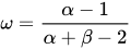
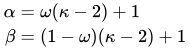
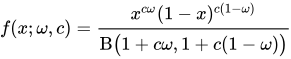
توزيعات بيتا المقعرة ، والتي تتميزيمكن تحديد معلمات ذلك من حيث النمط و"التركيز". النمط،والتركيز،ويمكن استخدامها لتحديد معلمات الشكل المعتادة على النحو التالي: [ 7 ] بالنسبة للوضع،لكي نكون محددين بشكل جيد، نحتاج إلىأو ما يعادل ذلكأما إذا عرّفنا التركيز على النحو التالي:، يتبسط الشرط إلىوكثافة بيتا عندويمكن كتابتها على النحو التالي: أينيقيس الإحصاءات الكافية بشكل مباشر ،ولاحظ أيضًا أنه في النهاية،يصبح التوزيع مسطحاً.










المتوسط والتباين
بحل نظام المعادلات (المترابطة) الواردة في الأقسام السابقة كمعادلات للمتوسط والتباين لتوزيع بيتا بدلالة المعلمات الأصلية α و β ، يمكن التعبير عن المعلمات α و β بدلالة المتوسط ( μ ) والتباين (var):
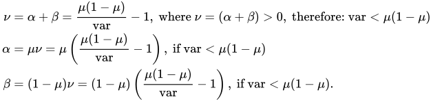
قد يؤدي هذا التحديد لمعاملات توزيع بيتا إلى فهم أكثر سهولة من الفهم القائم على المعاملات الأصلية α و β . على سبيل المثال، من خلال التعبير عن المنوال، والالتواء، والتفرطح الزائد، والإنتروبيا التفاضلية بدلالة المتوسط والتباين:


أربعة معايير
يتم دعم توزيع بيتا ذي معاملي الشكل α و β على النطاق [0,1] أو (0,1). من الممكن تغيير موقع ومقياس التوزيع عن طريق إدخال معاملين إضافيين يمثلان القيم الدنيا، a ، والقصوى ، c ( حيث c > a )، للتوزيع، [ 1 ] عن طريق تحويل خطي يستبدل المتغير غير البعدي x بدلالة المتغير الجديد y (الذي يدعم النطاق [ a , c ] أو ( a , c )) والمعاملين a و c .

دالة كثافة الاحتمال لتوزيع بيتا ذي الأربعة معلمات تساوي دالة كثافة الاحتمال لتوزيع ذي المعلمتين، مضروبة في المدى ( c - a )، (بحيث تكون المساحة الكلية تحت منحنى الكثافة مساوية لاحتمال واحد)، مع إزاحة المتغير "y" وقياسه على النحو التالي:
![{\displaystyle {\begin{aligned}f(y;\alpha ,\beta ,a,c)={\frac {f(x;\alpha ,\beta )}{ca}}&={\frac {\left({\frac {ya}{ca}}\right)^{\alpha -1}\left({\frac {cy}{ca}}\right)^{\beta -1}}{(ca)B(\alpha ,\beta )}}\\[1ex]&={\frac {(ya)^{\alpha -1}(cy)^{\beta -1}}{(ca)^{\alpha +\beta -1}B(\alpha ,\beta )}}.\end{aligned}}}](https://wikimedia.org/api/rest_v1/media/math/render/svg/ebfbb9c4da37593762747522d2d91a4ca72e0011)
يُرمز إلى أن المتغير العشوائي Y يتبع توزيع بيتا بأربعة معلمات α و β و a و c بالرمز التالي:

يتم تغيير مقياس بعض مقاييس الموقع المركزي (بواسطة ( c − a )) وإزاحتها (بواسطة a )، على النحو التالي:
![{\displaystyle {\begin{aligned}\mu _{Y}&=\mu _{X}(ca)+a\\[1ex]&={\frac {\alpha }{\alpha +\beta }}\left(ca\right)+a={\frac {\alpha c+\beta a}{\alpha +\beta }}\end{aligned}}}](https://wikimedia.org/api/rest_v1/media/math/render/svg/86a8b4fe30b5075b8c038d5b5b3e1f6ee8e5963f)
![{\displaystyle {\begin{aligned}{\text{mode}}(Y)&={\text{mode}}(X)(ca)+a\\[1ex]&={\frac {\alpha -1}{\alpha +\beta -2}}\left(ca\right)+a\\[1ex]&={\frac {(\alpha -1)c+(\beta -1)a}{\alpha +\beta -2}}\ ,&{\text{ إذا كان }}\alpha ,\,\beta >1\end{aligned}}}](https://wikimedia.org/api/rest_v1/media/math/render/svg/768c42362dbb2d2904c218dcfc6df1de62b5f635)
![{\displaystyle {\begin{aligned}{\text{median}}(Y)&={\text{median}}(X)(ca)+a\\[1ex]&=I_{\frac {1}{2}}^{[-1]}(\alpha ,\beta )\left(ca\right)+a\end{aligned}}}](https://wikimedia.org/api/rest_v1/media/math/render/svg/9b039773a1da5743c1e27109447176e3cfe1925e)
ملاحظة: لا يمكن تحويل المتوسط الهندسي والمتوسط التوافقي عن طريق التحويل الخطي بالطريقة التي يمكن بها تحويل المتوسط والوسيط والمنوال.
يمكن كتابة معلمات شكل Y بدلالة متوسطها وتباينها كما يلي:

يتم قياس مقاييس التشتت الإحصائي (لا تحتاج إلى إزاحة لأنها متمركزة بالفعل حول المتوسط) بواسطة المدى ( c − a )، خطيًا بالنسبة للانحراف المتوسط وغير خطيًا بالنسبة للتباين:
![{\displaystyle {\begin{aligned}&{\text{(الانحراف المتوسط حول المتوسط)}}(Y)\\[1ex]&=({\text{(الانحراف المتوسط حول المتوسط)}}(X))(ca)\\&={\frac {2\alpha ^{\alpha }\beta ^{\beta }}{\mathrm {B} (\alpha ,\beta )(\alpha +\beta )^{\alpha +\beta +1}}}(ca)\end{aligned}}}](https://wikimedia.org/api/rest_v1/media/math/render/svg/769fc1182a10805b989db4ae5c207769240dc3b5)

بما أن الالتواء والتفرطح الزائد كميتان لا بعديتان ( كلحظات متمركزة حول المتوسط ومُقاسة بالانحراف المعياري )، فإنهما مستقلتان عن المعاملين a و c ، وبالتالي فهما متساويتان مع التعبيرات المذكورة أعلاه بدلالة X (مع الدعم [0,1] أو (0,1)):

![{\displaystyle {\text{زيادة التفرطح}}(Y)={\text{زيادة التفرطح}}(X)={\frac {6\left[(\alpha -\beta )^{2}(\alpha +\beta +1)-\alpha \beta (\alpha +\beta +2)\right]}{\alpha \beta (\alpha +\beta +2)(\alpha +\beta +3)}}}](https://wikimedia.org/api/rest_v1/media/math/render/svg/76f8b524c994e9cdaf8317555457b4369ab2271e)
ملكيات
مقاييس النزعة المركزية
وضع
نمط المتغير العشوائي X الموزع بيتا مع α ، β > 1 هو القيمة الأكثر احتمالا للتوزيع (المقابلة للذروة في دالة كثافة الاحتمال)، ويتم إعطاؤه بالصيغة التالية: [ 1 ]

عندما تكون كلتا المعلمتين أقل من واحد ( α ، β < 1)، فهذا هو النمط المضاد: أدنى نقطة في منحنى كثافة الاحتمال. [ 8 ]
بوضع α = β ، يتبسط تعبير المنوال إلى 1/2، مما يدل على أنه عندما يكون α = β > 1، يكون المنوال (أو النمط المضاد عندما يكون α ، β < 1 ) في مركز التوزيع: وهو متناظر في هذه الحالات. راجع قسم الأشكال في هذه المقالة للاطلاع على قائمة كاملة بحالات المنوال، لقيم اختيارية لـ α و β . في العديد من هذه الحالات، تقع القيمة القصوى لدالة الكثافة عند أحد طرفي التوزيع أو كليهما. في بعض الحالات، تكون القيمة (القصوى) لدالة الكثافة عند الطرف محدودة. على سبيل المثال، في حالة α = 2، β = 1 (أو α = 1، β = 2)، تصبح دالة الكثافة توزيعًا مثلثيًا قائم الزاوية محدودًا عند كلا الطرفين. في حالات أخرى، توجد نقطة شاذة عند أحد الطرفين، حيث تقترب قيمة دالة الكثافة من اللانهاية. على سبيل المثال، في حالة α = β = 1/2، يتبسط توزيع بيتا ليصبح توزيع الجيب العكسي . يوجد جدل بين علماء الرياضيات حول بعض هذه الحالات، وما إذا كان يمكن تسمية طرفي التوزيع ( x = 0 و x = 1) بالمنوال أم لا. [ 9 ] [ 2 ]

متوسط


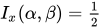
الوسيط لتوزيع بيتا هو العدد الحقيقي الفريدوالتي تكون دالة بيتا غير الكاملة المنتظمة لهالا توجد صيغة عامة مغلقة لوسيط توزيع بيتا لأي قيم لـ α و β . فيما يلي صيغ مغلقة لقيم محددة للمعاملين α و β :
![{\displaystyle x=I_{1/2}^{[-1]}(\alpha ,\beta )}](https://wikimedia.org/api/rest_v1/media/math/render/svg/d7510f94efa49f254eb3924678b527a6fd22d0fc)
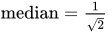
- في الحالات المتناظرة α = β ، الوسيط = 1/2.
- بالنسبة لـ α = 1 و β > 0، الوسيط(هذه الحالة هي صورة معكوسة لتوزيع دالة القوة )
- بالنسبة لـ α > 0 و β = 1، الوسيط =(هذه الحالة هي توزيع دالة القوة [ 9 ] )
- بالنسبة لـ α = 3 و β = 2، الوسيط = 0.6142724318676105...، الحل الحقيقي للمعادلة الرباعية 1 − 8 x 3 + 6 x 4 = 0، والتي تقع في [0,1].
- بالنسبة لـ α = 2 و β = 3، الوسيط = 0.38572756813238945... = 1−median(Beta(3, 2))


فيما يلي الحدود التي يكون فيها أحد المعاملات محدودًا (غير صفري) والآخر يقترب من هذه الحدود:
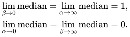
يتم إعطاء تقريب معقول لقيمة الوسيط لتوزيع بيتا، لكل من α و β أكبر من أو يساوي واحد، بواسطة الصيغة [ 10 ].
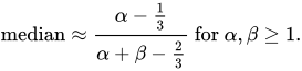
عندما تكون قيمتا α و β أكبر من أو تساوي 1، يكون الخطأ النسبي ( الخطأ المطلق مقسومًا على الوسيط) في هذا التقريب أقل من 4%، ويكون أقل من 1% عندما تكون قيمتا α و β أكبر من أو تساويان 2 أو أكبر من أو تساويان 2. وبالمثل، يكون الخطأ المطلق مقسومًا على الفرق بين المتوسط والمنوال صغيرًا جدًا.


يقصد

القيمة المتوقعة (المتوسط) ( μ ) لمتغير عشوائي X ذي توزيع بيتا مع معلمتين α و β هي دالة لنسبة β / α لهذه المعلمات فقط: [ 1 ]
![\begin{aligned}\mu =\operatorname {E} [X]&=\int _{0}^{1}xf(x;\alpha ,\beta )\,dx\\&=\int _{0}^{1}x\,{\frac {x^{\alpha -1}(1-x)^{\beta -1}}{\mathrm {B} (\alpha ,\beta )}}\,dx\\&={\frac {\alpha }{\alpha +\beta }}\\&={\frac {1}{1+{\frac {\beta }{\alpha }}}}\end{aligned}}}](https://wikimedia.org/api/rest_v1/media/math/render/svg/e9137834d9d47360ed6c23550c6236fed5fd35f7)
بوضع α = β في المعادلة أعلاه، نحصل على μ = 1/2 ، مما يدل على أن المتوسط، عندما α = β، يقع في مركز التوزيع: أي أنه متماثل. كما يمكن استنتاج النهايات التالية من المعادلة أعلاه:

لذا، عندما تقترب نسبة β / α من الصفر، أو عندما تقترب نسبة α / β من اللانهاية، يقع المتوسط عند الطرف الأيمن، x = 1. عند هذه النسب الحدية، يصبح توزيع بيتا توزيعًا منحلًا بنقطة واحدة مع ذروة دالة ديراك دلتا عند الطرف الأيمن، x = 1 ، باحتمالية 1، واحتمالية صفرية في أي مكان آخر. هناك احتمالية 100% (يقين مطلق) مركزة عند الطرف الأيمن، x = 1 .
وبالمثل، عندما تؤول نسبة β / α إلى اللانهاية، أو عندما تؤول نسبة α / β إلى الصفر، يقع المتوسط عند الطرف الأيسر، x = 0. يصبح توزيع بيتا توزيعًا منحلًا بنقطة واحدة مع ذروة دالة ديراك دلتا عند الطرف الأيسر، x = 0، باحتمالية 1، واحتمالية صفرية في أي مكان آخر. هناك احتمالية 100% (يقين مطلق) مركزة عند الطرف الأيسر، x = 0. فيما يلي النهايات عندما تكون إحدى المعلمتين محدودة (غير صفرية) والأخرى تقترب من هذه النهايات:

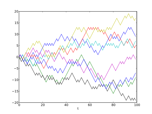
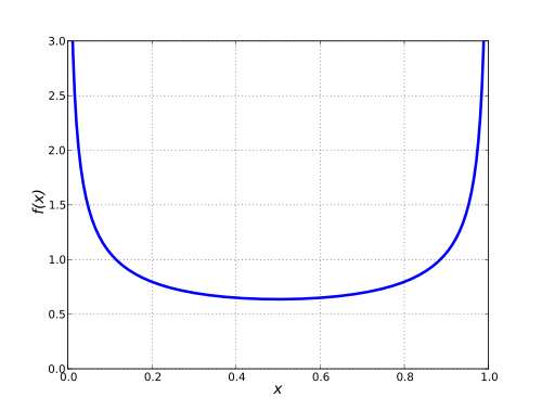
في حين أنه من المعروف أن متوسط العينة (كتقدير للموقع) ليس بنفس قوة الوسيط في التوزيعات أحادية النمط النموذجية (ذات الأنماط المركزية، ونقاط الانعطاف على جانبي النمط، والذيل الطويل) ( حيث α و β > 2 ) ، فإن العكس صحيح في التوزيعات ثنائية النمط المنتظمة أو "على شكل حرف U" (حيث α و β ≤ 1 ) ، إذ تقع الأنماط عند طرفي التوزيع. وكما أشار موستيلر وتوكي ( [ 11 ] ، ص 207) : " يستخدم متوسط القيمتين المتطرفتين جميع معلومات العينة. وهذا يوضح كيف ينبغي أن تحظى القيم المتطرفة بوزن أكبر في التوزيعات قصيرة الذيل." على النقيض من ذلك، يتضح أن الوسيط للتوزيعات ثنائية النمط "على شكل حرف U" ذات الأنماط عند حافة التوزيع (مع Beta( α , β ) بحيث α , β ≤ 1 ) ليس متينًا، لأن وسيط العينة يستبعد المشاهدات المتطرفة من العينة. ويظهر تطبيق عملي لهذا، على سبيل المثال، في المسارات العشوائية ، حيث أن احتمال وقت آخر زيارة لنقطة الأصل في مسار عشوائي يتوزع وفقًا لتوزيع دالة الجيب العكسي Beta(1/2, 1/2): [ 5 ] [ 12 ] وبالتالي، فإن متوسط عدد من عمليات محاكاة المسار العشوائي يُعدّ مقدرًا أكثر متانة من الوسيط (الذي يُعدّ تقديرًا غير مناسب لحجم العينة في هذه الحالة).
المتوسط الهندسي


إن لوغاريتم المتوسط الهندسي G X لتوزيع ذي متغير عشوائي X هو المتوسط الحسابي لـ ln( X )، أو بشكل مكافئ، قيمته المتوقعة:
![{\displaystyle \ln G_{X}=\operatorname {E} [\ln X]}](https://wikimedia.org/api/rest_v1/media/math/render/svg/64b67cb73b90bc0e09ba41003b44f84b6e1d3feb)
بالنسبة لتوزيع بيتا، فإن تكامل القيمة المتوقعة يعطي:
![\begin{aligned}\operatorname {E} [\ln X]&=\int _{0}^{1}\ln x\,f(x;\alpha ,\beta )\,dx\\[4pt]&=\int _{0}^{1}\ln x\,{\frac {x^{\alpha -1}(1-x)^{\beta -1}}{\mathrm {B} (\alpha ,\beta )}}\,dx\\[4pt]&={\frac {1}{\mathrm {B} (\alpha ,\beta )}}\,\int _{0}^{1}{\frac {\partial x^{\alpha -1}(1-x)^{\beta -1}}{\partial \alpha }}\,dx\\[4pt]&={\frac {1}{\mathrm {B} \int_{0}^{1}x^{\alpha -1}(1-x)^{\beta -1}\,dx\\[4pt]&={\frac{1}{\mathrm{B}(\alpha,\beta)}}{\frac{\partial\mathrm{B}(\alpha,\beta)}{\partial\alpha}}\\[4pt]&={\frac{\partial\ln\mathrm{B}(\alpha,\beta)}{\partial\alpha}}\\[4pt]&={\frac{\partial\ln\Gamma(\alpha)}{\partial\alpha}}-{\frac{\partial\ln\Gamma(\alpha +\beta)}{\partial \alpha }}\\[4pt]&=\psi (\alpha )-\psi (\alpha +\beta )\end{aligned}}}](https://wikimedia.org/api/rest_v1/media/math/render/svg/cd9db519e08e3c72cd6f9e2f0c90a7c57bdba035)
حيث ψ هي دالة ديغاما .
لذلك، فإن المتوسط الهندسي لتوزيع بيتا ذي معلمات الشكل α و β هو الدالة الأسية لدوال ديغاما لـ α و β كما يلي:
![{\displaystyle G_{X}=e^{\operatorname {E} [\ln X]}=e^{\psi (\alpha )-\psi (\alpha +\beta )}}](https://wikimedia.org/api/rest_v1/media/math/render/svg/c93ffa7f0155fa3816fcb151c3eb677700aabca2)
في حين أنه بالنسبة لتوزيع بيتا ذي معاملات شكل متساوية α = β ، فإن معامل الالتواء يساوي صفرًا، والمنوال يساوي المتوسط ويساوي الوسيط ويساوي 1/2، فإن المتوسط الهندسي يكون أقل من 1/2: 0 < G X < 1/2 . والسبب في ذلك هو أن التحويل اللوغاريتمي يُرجّح بشدة قيم X القريبة من الصفر، حيث يميل ln( X ) بشدة نحو سالب ما لا نهاية عندما تقترب X من الصفر، بينما يتسطح ln( X ) نحو الصفر عندما X → 1 .
على طول الخط α = β ، تنطبق الحدود التالية:
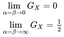
فيما يلي الحدود مع وجود أحد المعاملات محدودًا (غير صفري) والآخر يقترب من هذه الحدود:
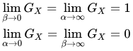
يُظهر الرسم البياني المرفق الفرق بين المتوسط والمتوسط الهندسي لمعاملات الشكل α و β من الصفر إلى 2. وبالإضافة إلى حقيقة أن الفرق بينهما يقترب من الصفر عندما تقترب α و β من اللانهاية، وأن هذا الفرق يصبح كبيرًا عندما تقترب قيم α و β من الصفر، يمكن ملاحظة عدم تناظر واضح في المتوسط الهندسي بالنسبة لمعاملات الشكل α و β . ويكون الفرق بين المتوسط الهندسي والمتوسط أكبر عند القيم الصغيرة لـ α مقارنةً بـ β منه عند تبديل قيم β و α .
يقترح كل من NLJohnson و S. Kotz [ 1 ] التقريب اللوغاريتمي لدالة ديجاما ψ ( α ) ≈ ln( α − 1/2) والذي ينتج عنه التقريب التالي للمتوسط الهندسي:
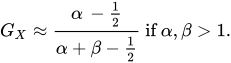
فيما يلي القيم الرقمية للخطأ النسبي في هذا التقريب: [ ( α = β = 1): 9.39% ]؛ [ ( α = β = 2): 1.29% ]; [ ( α = 2، β = 3): 1.51% ]؛ [ ( α = 3، β = 2): 0.44% ]؛ [ ( α = β = 3): 0.51% ]; [ ( α = β = 4): 0.26% ]; [ ( α = 3، β = 4): 0.55% ]؛ [ ( α = 4, β = 3): 0.24% ].
وبالمثل، يمكن حساب قيمة معلمات الشكل اللازمة لكي يساوي المتوسط الهندسي 1/2. بمعرفة قيمة المعلمة β ، ما هي قيمة المعلمة الأخرى α اللازمة لكي يساوي المتوسط الهندسي 1/2؟ الجواب هو أنه (عندما تكون β > 1 )، فإن قيمة α المطلوبة تقترب من β + 1/2 عندما تقترب β من اللانهاية . على سبيل المثال، كل هذه الأزواج لها نفس الوسط الهندسي 1/2: [ β = 1, α = 1.4427 ], [ β = 2, α = 2.46958 ], [ β = 3, α = 3.47943 ], [ β = 4, α = 4.48449 ], [ β = 5, α = 5.48756 ]، [ β = 10، α = 10.4938 ]، [ β = 100، α = 100.499 ].
الخاصية الأساسية للمتوسط الهندسي، والتي يمكن إثبات عدم صحتها لأي متوسط آخر، هي

هذا يجعل المتوسط الهندسي المتوسط الصحيح الوحيد عند حساب متوسط النتائج المعيارية ، أي النتائج المعروضة كنسب إلى القيم المرجعية. [ 13 ] وهذا مهم لأن توزيع بيتا نموذج مناسب للسلوك العشوائي للنسب المئوية، وهو مناسب بشكل خاص للنمذجة الإحصائية للنسب. يلعب المتوسط الهندسي دورًا محوريًا في تقدير الاحتمال الأقصى، انظر قسم "تقدير المعلمات، الاحتمال الأقصى". في الواقع، عند إجراء تقدير الاحتمال الأقصى، بالإضافة إلى المتوسط الهندسي G( X) القائم على المتغير العشوائي X، يظهر أيضًا متوسط هندسي آخر بشكل طبيعي: المتوسط الهندسي القائم على التحويل الخطي – (1 − X ) ، وهو صورة معكوسة لـ X ، ويرمز له بـ G (1 − X ) .
![{\displaystyle G_{1-X}=e^{\operatorname {E} [\ln(1-X)]}=e^{\psi (\beta ) -\psi (\alpha +\beta )}}](https://wikimedia.org/api/rest_v1/media/math/render/svg/58d36e067302e87f85db3f0fb1e2902201e38d76)
على طول الخط α = β ، تنطبق الحدود التالية:

فيما يلي الحدود مع وجود أحد المعاملات محدودًا (غير صفري) والآخر يقترب من هذه الحدود:
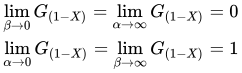
تبلغ قيمتها التقريبية ما يلي:
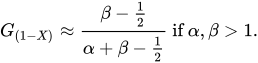
على الرغم من أن كلاً من G X و G 1− X غير متناظرين، إلا أنه في حالة تساوي معاملي الشكل α = β ، فإن المتوسطات الهندسية متساوية: G X = G (1− X ) . وتنتج هذه المساواة من التناظر التالي بين المتوسطين الهندسيين:

المتوسط التوافقي


مقلوب المتوسط التوافقي ( H<sub> X </sub>) لتوزيع ذي متغير عشوائي X هو المتوسط الحسابي لـ 1/ X ، أو ما يعادله، قيمته المتوقعة. لذا، فإن المتوسط التوافقي ( H <sub>X</sub> ) لتوزيع بيتا ذي معاملي الشكل α و β هو:
![{\displaystyle {\begin{aligned}H_{X}&={\frac {1}{\operatorname {E} \left[{\frac {1}{X}}\right]}}\\&={\frac {1}{\int _{0}^{1}{\frac {f(x;\alpha ,\beta )}{x}}\,dx}}\\&={\frac {1}{\int _{0}^{1}{\frac {x^{\alpha -1}(1-x)^{\beta -1}}{x\mathrm {B} (\alpha ,\beta )}}\,dx}}\\&={\frac {\alpha -1}{\alpha +\beta -1}}{\text{ إذا كان }}\alpha >1{\text{ و }}\beta >0\\\end{aligned}}}](https://wikimedia.org/api/rest_v1/media/math/render/svg/ed7d99dd7493b9c085cd5d407861730e2a2abf6c)
المتوسط التوافقي ( H X ) لتوزيع بيتا مع α < 1 غير معرف، لأن تعبيره المحدد غير محدود في [0، 1] لمعامل الشكل α أقل من واحد.
بوضع α = β في التعبير أعلاه، نحصل على
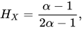
مما يدل على أنه بالنسبة لـ α = β يتراوح المتوسط التوافقي من 0، بالنسبة لـ α = β = 1، إلى 1/2، بالنسبة لـ α = β → ∞.
فيما يلي الحدود مع وجود أحد المعاملات محدودًا (غير صفري) والآخر يقترب من هذه الحدود:
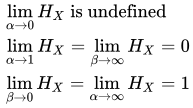
يلعب المتوسط التوافقي دورًا في تقدير الاحتمال الأقصى لحالة المعلمات الأربع، بالإضافة إلى المتوسط الهندسي. في الواقع، عند إجراء تقدير الاحتمال الأقصى لحالة المعلمات الأربع، إلى جانب المتوسط التوافقي H X القائم على المتغير العشوائي X ، يظهر أيضًا متوسط توافقي آخر بشكل طبيعي: المتوسط التوافقي القائم على التحويل الخطي (1 − X )، وهو صورة معكوسة لـ X ، ويرمز له بـ H 1 − X.
![{\displaystyle H_{1-X}={\frac {1}{\operatorname {E} \left[{\frac {1}{1-X}}\right]}}={\frac {\beta -1}{\alpha +\beta -1}}{\text{ إذا كان }}\beta >1،{\text{ و }}\alpha >0.}](https://wikimedia.org/api/rest_v1/media/math/render/svg/48f4fd69f20c4259cb8a50e754df8dfed5a1ddca)
المتوسط التوافقي ( H (1 − X ) ) لتوزيع بيتا مع β < 1 غير معرف، لأن تعبيره المحدد غير محدود في [0، 1] لمعامل الشكل β أقل من واحد.
بوضع α = β في التعبير أعلاه، نحصل على
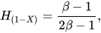
مما يدل على أنه بالنسبة لـ α = β يتراوح المتوسط التوافقي من 0، بالنسبة لـ α = β = 1، إلى 1/2، بالنسبة لـ α = β → ∞.
فيما يلي الحدود مع وجود أحد المعاملات محدودًا (غير صفري) والآخر يقترب من هذه الحدود:
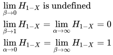
على الرغم من أن كلاً من H X و H 1− X غير متناظرين، فإنه في حالة تساوي معاملي الشكل α = β ، تتساوى المتوسطات التوافقية: H X = H 1− X. وتنتج هذه المساواة من التناظر التالي بين المتوسطين التوافقيين:

مقاييس التشتت الإحصائي
التباين
التباين (العزم الثاني المتمركز حول المتوسط) لمتغير عشوائي X ذي توزيع بيتا مع المعلمات α و β هو : [ 1 ] [ 14 ]
![{\displaystyle \operatorname {var} (X)=\operatorname {E} \left[(X-\mu )^{2}\right]={\frac {\alpha \beta }{\left(\alpha +\beta \right)^{2}\left(\alpha +\beta +1\right)}}}](https://wikimedia.org/api/rest_v1/media/math/render/svg/d7d2effe47b57f9a004264ee6aac04029d3954de)
بوضع α = β في التعبير أعلاه، نحصل على
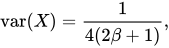
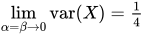
يُظهر هذا أنه عندما α = β، يتناقص التباين بشكل رتيب مع ازدياد α = β . بوضع α = β = 0 في هذه المعادلة، نجد أن أقصى تباين var( X ) = 1/4 [ 1 ] لا يحدث إلا عند الاقتراب من النهاية، أي عند α = β = 0 .
يمكن أيضًا تحديد معلمات توزيع بيتا من حيث متوسطه μ (0 < μ < 1) وحجم العينة ν = α + β ( ν > 0 ) (انظر القسم الفرعي المتوسط وحجم العينة ):

باستخدام هذه المعلمة ، يمكن التعبير عن التباين بدلالة المتوسط μ وحجم العينة ν على النحو التالي:
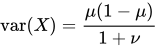
بما أن ν = α + β > 0 ، فإنه يتبع ذلك var( X ) < μ (1 − μ ) .
بالنسبة للتوزيع المتماثل، يكون المتوسط في منتصف التوزيع، μ = 1/2 ، وبالتالي:
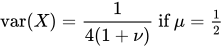
كذلك، يمكن الحصول على النهايات التالية (مع اقتراب المتغير المذكور فقط من النهاية) من التعبيرات المذكورة أعلاه:


التباين والتباين المشترك الهندسي


إن لوغاريتم التباين الهندسي، ln(var GX )، لتوزيع ذي متغير عشوائي X هو العزم الثاني للوغاريتم X متمركزًا حول المتوسط الهندسي لـ X ، ln( G X ):
![{\displaystyle {\begin{aligned}\ln \operatorname {var} _{GX}&=\operatorname {E} \left[\left(\ln X-\ln G_{X}\right)^{2}\right]\\&=\operatorname {E} \left[\left(\ln X-\operatorname {E} \left[\ln X\right]\right)^{2}\right]\\&=\operatorname {E} \left[\left(\ln X\right)^{2}\right]-\left(\operatorname {E} [\ln X]\right)^{2}\\&=\operatorname {var} [\ln X]\end{aligned}}}](https://wikimedia.org/api/rest_v1/media/math/render/svg/03642aabe02f83fe6e01e5a136c245d82b898904)
وبالتالي، فإن التباين الهندسي هو:
![{\displaystyle \operatorname {var} _{GX}=e^{\operatorname {var} [\ln X]}}](https://wikimedia.org/api/rest_v1/media/math/render/svg/524cf664ccfd5eb381fd1987926209f1c401a200)
في مصفوفة معلومات فيشر ، وانحناء دالة الاحتمال اللوغاريتمي، يظهر لوغاريتم التباين الهندسي للمتغير المنعكس 1 − X ولوغاريتم التغاير الهندسي بين X و 1 − X :
![\displaystyle \begin{aligned}\ln \operatorname {var_{G(1-X)}} &=\operatorname {E} \left[\left(\ln(1-X)-\ln G_{1-X}\right)^{2}\right]\\&=\operatorname {E} \left[\left(\ln(1-X)-\operatorname {E} [\ln(1-X)]\right)^{2}\right]\\&=\operatorname {E} \left[(\ln(1-X))^{2}\right]-\left(\operatorname {E} [\ln(1-X)]\right)^{2}\\&=\operatorname {var} [\ln(1-X)]\\&\\\operatorname {var_{G(1-X)}} &=e^{\operatorname {var} [\ln(1-X)]}\\&\\\ln \operatorname {cov_{G{X,1-X}}} &=\operatorname {E} [(\ln X-\ln G_{X})(\ln(1-X)-\ln G_{1-X})]\\&=\اسم المشغل {E} [(\ln X-\اسم المشغل {E} [\ln X])(\ln(1-X)-\operatorname {E} [\ln(1-X)])]\\&=\operatorname {E} \left[\ln X\ln(1-X)\right]-\operatorname {E} [\ln X]\operatorname {E} [\ln(1-X)]\\&=\اسم المشغل {cov} [\ln X,\ln(1-X)]\\&\\\اسم المشغل {cov} _ {G{X,(1-X)}}&=e^{\operatorname {cov} [\ln X,\ln(1-X)]}\end{محاذاة}}}](https://wikimedia.org/api/rest_v1/media/math/render/svg/657c11ca41846366cb8d9843536af9e002ea4cdf)
بالنسبة لتوزيع بيتا، يمكن اشتقاق العزوم اللوغاريتمية من الرتب العليا باستخدام تمثيل توزيع بيتا كنسبة من توزيعين غاما، ثم اشتقاق التكامل. ويمكن التعبير عنها بدلالة دوال غاما متعددة الرتب العليا. انظر القسم § عزوم المتغيرات العشوائية المحولة لوغاريتميًا . تباين المتغيرات اللوغاريتمية والتباين المشترك لـ ln X و ln(1− X ) هما:
![{\displaystyle \operatorname {var} [\ln X]=\psi _{1}(\alpha )-\psi _{1}(\alpha +\beta )}](https://wikimedia.org/api/rest_v1/media/math/render/svg/e396e8700267735eb741f73e8906445579c43bc6)
![{\displaystyle \operatorname {var} [\ln(1-X)]=\psi _{1}(\beta )-\psi _{1}(\alpha +\beta )}](https://wikimedia.org/api/rest_v1/media/math/render/svg/70eefadef46c7d56cc13c8221aa3df1d71596b7f)
![{\displaystyle \operatorname {cov} [\ln X,\ln(1-X)]=-\psi _{1}(\alpha +\beta )}](https://wikimedia.org/api/rest_v1/media/math/render/svg/e7a515ada0b9d62c5a3a7b35662b03256d66e3b9)
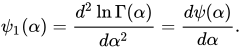
حيث أن دالة تريغاما ، التي يرمز لها بـ ψ 1 ( α )، هي الثانية من دوال بوليغاما ، وتُعرف بأنها مشتقة دالة ديغاما :
لذلك،
![{\displaystyle \ln \operatorname {var} _{GX}=\operatorname {var} [\ln X]=\psi _{1}(\alpha )-\psi _{1}(\alpha +\beta )}](https://wikimedia.org/api/rest_v1/media/math/render/svg/194b00552edda5d8d026a24872cdb27b604516c9)
![{\displaystyle \ln \operatorname {var} _{G(1-X)}=\operatorname {var} [\ln(1-X)]=\psi _{1}(\beta )-\psi _{1}(\alpha +\beta )}](https://wikimedia.org/api/rest_v1/media/math/render/svg/96dd82553307c025c84da68a3c373aad7467abd2)
![{\displaystyle \ln \operatorname {cov} _{GX,1-X}=\operatorname {cov} [\ln X,\ln(1-X)]=-\psi _{1}(\alpha +\beta )}](https://wikimedia.org/api/rest_v1/media/math/render/svg/40a793c0271e457f671edb0668edc15bbae8740f)
تُظهر الرسوم البيانية المرفقة التباينات الهندسية اللوغاريتمية والتباين المشترك الهندسي اللوغاريتمي مقابل معاملي الشكل α و β . وتُبين هذه الرسوم أن التباينات الهندسية اللوغاريتمية والتباين المشترك الهندسي اللوغاريتمي يقتربان من الصفر عندما يكون معاملا الشكل α و β أكبر من 2، وأن التباينات الهندسية اللوغاريتمية ترتفع بسرعة عندما يكون معاملا الشكل α و β أقل من 1. وتكون التباينات الهندسية اللوغاريتمية موجبة لجميع قيم معاملي الشكل. أما التباين المشترك الهندسي اللوغاريتمي فهو سالب لجميع قيم معاملي الشكل، ويصل إلى قيم سالبة كبيرة عندما يكون α و β أقل من 1.
فيما يلي الحدود مع وجود أحد المعاملات محدودًا (غير صفري) والآخر يقترب من هذه الحدود:

الحدود مع تغير معيارين:

على الرغم من أن كلاً من ln(var GX ) و ln(var G (1 − X ) ) غير متناظرين، إلا أنه عندما تتساوى معاملات الشكل، α = β ، نحصل على: ln(var GX ) = ln(var G (1− X ) ). وتنتج هذه المساواة من التناظر التالي بين التباينين الهندسيين اللوغاريتميين:

التغاير الهندسي اللوغاريتمي متناظر:

متوسط الانحراف المطلق حول المتوسط


الانحراف المطلق المتوسط حول المتوسط لتوزيع بيتا بمعاملات الشكل α و β هو: [ 9 ]
![{\displaystyle \operatorname {E} [|XE[X]|]={\frac {2\alpha ^{\alpha }\beta ^{\beta }}{\mathrm {B} (\alpha ,\beta )(\alpha +\beta )^{\alpha +\beta +1}}}}](https://wikimedia.org/api/rest_v1/media/math/render/svg/6d1c6330a91df22b40cedc7903dbc70120d66cf9)
يُعدّ متوسط الانحراف المطلق حول المتوسط مقياسًا أكثر دقةً للتشتت الإحصائي من الانحراف المعياري لتوزيعات بيتا ذات الذيول ونقاط الانعطاف على جانبي المنوال، أي توزيعات بيتا ( α , β ) حيث α و β > 2، لأنه يعتمد على الانحرافات الخطية (المطلقة) بدلًا من الانحرافات التربيعية عن المتوسط. ولذلك، لا يُؤخذ تأثير الانحرافات الكبيرة جدًا عن المتوسط في الحسبان بنفس القدر.
باستخدام تقريب ستيرلينغ لدالة غاما ، اشتق كل من NLJohnson و S.Kotz [ 1 ] التقريب التالي لقيم معلمات الشكل الأكبر من واحد (الخطأ النسبي لهذا التقريب هو -3.5% فقط لـ α = β = 1، ويتناقص إلى الصفر عندما α → ∞، β → ∞):
![{\displaystyle {\begin{aligned}{\frac {\text{الانحراف المطلق المتوسط عن المتوسط}}{\text{الانحراف المعياري}}}&={\frac {\operatorname {E} [|XE[X]|]}{\sqrt {\operatorname {var} (X)}}}\\&\approx {\sqrt {\frac {2}{\pi }}}\left(1+{\frac {7}{12(\alpha +\beta )}}{}-{\frac {1}{12\alpha }}-{\frac {1}{12\beta }}\right),{\text{ إذا كان }}\alpha ,\beta >1.\end{aligned}}}](https://wikimedia.org/api/rest_v1/media/math/render/svg/c196a5a2eb110b71471a3dc019241c6cb8c3f927)
عند الحد α → ∞، β → ∞، تصبح نسبة الانحراف المطلق المتوسط إلى الانحراف المعياري (لتوزيع بيتا) مساوية لنسبة نفس المقاييس للتوزيع الطبيعي:عندما تكون α = β = 1، فإن هذه النسبة تساويوبالتالي، من α = β = 1 إلى α , β → ∞، تنخفض النسبة بنسبة 8.5%. أما عند α = β = 0، فإن الانحراف المعياري يساوي تمامًا متوسط الانحراف المطلق حول المتوسط. لذلك، تنخفض هذه النسبة بنسبة 15% من α = β = 0 إلى α = β = 1، وبنسبة 25% من α = β = 0 إلى α , β → ∞. مع ذلك، بالنسبة لتوزيعات بيتا الملتوية حيث α → 0 أو β → 0، تقترب نسبة الانحراف المعياري إلى متوسط الانحراف المطلق من اللانهاية (مع أن كلًا منهما، على حدة، يقترب من الصفر) لأن متوسط الانحراف المطلق يقترب من الصفر أسرع من الانحراف المعياري.


باستخدام المعلمات من حيث المتوسط μ وحجم العينة ν = α + β > 0:
يمكن التعبير عن متوسط الانحراف المطلق حول المتوسط بدلالة المتوسط μ وحجم العينة ν على النحو التالي:
![{\displaystyle \operatorname {E} [|XE[X]|]={\frac {2\mu ^{\mu \nu }(1-\mu )^{(1-\mu )\nu }}{\nu \mathrm {B} (\mu \nu ,(1-\mu )\nu )}}}](https://wikimedia.org/api/rest_v1/media/math/render/svg/027efecf8aaefea8c805194e47a1374ffcb63cb8)
بالنسبة للتوزيع المتماثل، يكون المتوسط في منتصف التوزيع، μ = 1/2، وبالتالي:
![{\displaystyle {\begin{align}\operatorname {E} [|XE[X]|]={\frac {2^{1-\nu }}{\nu \mathrm {B} ({\tfrac {\nu }{2}},{\tfrac {\nu }{2}})}}&= {\frac {2^{1-\nu }\Gamma (\nu )}{\nu (\Gamma) ({\tfrac {\nu }{2}}))^{2}}}\\\lim _{\nu \to 0}\left(\lim _{\mu \to {\frac {1}{2}}}\operatorname {E} [|XE[X]|]\right)&={\frac {1}{2}}\\\lim _{\nu \to \infty }\left(\lim _{\mu \to {\frac {1}{2}}}\operatorname {E} [|XE[X]|]\right)&=0\end{aligned}}}](https://wikimedia.org/api/rest_v1/media/math/render/svg/745a053a1ef3cc7edf07332763b401bd09b40e42)
كذلك، يمكن الحصول على النهايات التالية (مع اقتراب المتغير المذكور فقط من النهاية) من التعبيرات المذكورة أعلاه:
![{\displaystyle {\begin{aligned}\lim _{\beta \to 0}\operatorname {E} [|XE[X]|]&=\lim _{\alpha \to 0}\operatorname {E} [|XE[X]|]=0\\\lim _{\beta \to \infty }\operatorname {E} [|XE[X]|]&=\lim _{\alpha \to \infty }\operatorname {E} [|XE[X]|]=0\\\lim _{\mu \to 0}\operatorname {E} [|XE[X]|]&=\lim _{\mu \to 1}\operatorname {E} [|XE[X]|]=0\\\lim _{\nu \to 0}\operatorname {E} [|XE[X]|]&={\sqrt {\mu (1-\mu )}}\\\lim _{\nu \to \infty }\operatorname {E} [|XE[X]|]&=0\end{aligned}}}](https://wikimedia.org/api/rest_v1/media/math/render/svg/87c43b4a05f8ea3acf3f15b0a16f6ee07811ac6b)
متوسط الفرق المطلق
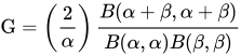
متوسط الفرق المطلق لتوزيع بيتا هو:
![{\displaystyle {\begin{aligned}\mathrm {MD} &=\int _{0}^{1}\int _{0}^{1}f(x;\alpha ,\beta )\,f(y;\alpha ,\beta )\left|xy\right|dx\,dy\\[1ex]&={\frac {4}{\alpha +\beta }}{\frac {B(\alpha +\beta ,\alpha +\beta )}{B(\alpha ,\alpha )B(\beta ,\beta )}}\end{aligned}}}](https://wikimedia.org/api/rest_v1/media/math/render/svg/0de290eea66b8a424727bff1b9a02f53f2607361)
معامل جيني لتوزيع بيتا يساوي نصف متوسط الفرق المطلق النسبي:
الانحراف

إن معامل الالتواء (العزم الثالث المتمركز حول المتوسط، مقومًا على أساس قوة التباين 3/2) لتوزيع بيتا هو [ 1 ]
![{\displaystyle \gamma _{1}={\frac {\operatorname {E} \left[\left(X-\mu \right)^{3}\right]}{\left(\operatorname {var} (X)\right)^{3/2}}}={\frac {2\left(\beta -\alpha \right){\sqrt {\alpha +\beta +1}}}{\left(\alpha +\beta +2\right){\sqrt {\alpha \beta }}}}.}](https://wikimedia.org/api/rest_v1/media/math/render/svg/1c880f0b8322d91fe382f87eaa4f8730faa164ed)
بوضع α = β في التعبير أعلاه، نحصل على γ 1 = 0، مما يُظهر مرة أخرى أن التوزيع متماثل عندما α = β ، وبالتالي فإن معامل الالتواء يساوي صفرًا. يكون الالتواء موجبًا (ذيل أيمن) عندما α < β ، وسالبًا (ذيل أيسر) عندما α > β .
باستخدام المعلمات من حيث المتوسط μ وحجم العينة ν = α + β :
يمكن التعبير عن الالتواء بدلالة المتوسط μ وحجم العينة ν على النحو التالي:
![{\displaystyle \gamma _{1}={\frac {\operatorname {E} [(X-\mu )^{3}]}{\left(\operatorname {var} (X)\right)^{3/2}}}={\frac {2(1-2\mu ){\sqrt {1+\nu }}}{(2+\nu ){\sqrt {\mu (1-\mu )}}}}.}](https://wikimedia.org/api/rest_v1/media/math/render/svg/c88399efb587f7d2443ddb232e4b24f2763050b9)
ويمكن التعبير عن معامل الالتواء أيضاً بدلالة التباين var والمتوسط μ كما يلي:
![{\displaystyle \gamma _{1}={\frac {\operatorname {E} [(X-\mu )^{3}]}{(\operatorname {var} (X))^{3/2}}}={\frac {2(1-2\mu ){\sqrt {\operatorname {var} }}}{\mu (1-\mu )+\operatorname {var} }}{\text{ إذا كان }}\operatorname {var} <\mu (1-\mu )}](https://wikimedia.org/api/rest_v1/media/math/render/svg/6b48373ac7ce8096381e7f74edf9e44bc435ad13)
يوضح الرسم البياني المصاحب للالتواء كدالة للتباين والمتوسط أن أقصى تباين (1/4) مقترن بالتواء صفري وشرط التناظر ( μ = 1/2)، وأن أقصى التواء (ما لا نهاية موجبة أو سالبة) يحدث عندما يكون المتوسط موجودًا في أحد الطرفين أو الآخر، بحيث تتركز "كتلة" توزيع الاحتمالية عند الأطراف (أدنى تباين).
يُعد التعبير التالي لمربع الالتواء، بدلالة حجم العينة ν = α + β والتباين var، مفيدًا لتقدير طريقة العزوم لأربعة معلمات:
![{\displaystyle (\gamma _{1})^{2}={\frac {\left(\operatorname {E} [(X-\mu )^{3}]\right)^{2}}{\left(\operatorname {var} (X)\right)^{3}}}={\frac {4}{(2+\nu )^{2}}}\left({\frac {1}{\operatorname {var} }}-4(1+\nu )\right)}](https://wikimedia.org/api/rest_v1/media/math/render/svg/b4f7b7d9a6d73e9bbcc43812b8f3fd573bc02ee3)
هذا التعبير يعطي بشكل صحيح قيمة انحراف تساوي صفرًا لـ α = β ، لأنه في هذه الحالة (انظر § التباين ):.

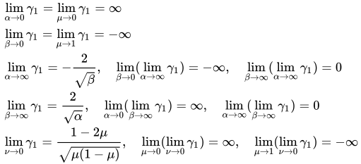
في حالة التناظر ( α = β )، يكون الانحراف = 0 على كامل النطاق، وتنطبق الحدود التالية:

بالنسبة للحالات غير المتماثلة ( α ≠ β )، يمكن الحصول على النهايات التالية (مع اقتراب المتغير المذكور فقط من النهاية) من التعبيرات أعلاه:


التفرطح

استُخدم توزيع بيتا في التحليل الصوتي لتقييم تلف التروس، إذ يُعدّ تفرطح توزيع بيتا مؤشرًا جيدًا لحالة الترس. [ 15 ] كما استُخدم التفرطح لتمييز الإشارة الزلزالية الناتجة عن خطوات الإنسان عن الإشارات الأخرى. فبما أن الأشخاص أو الأهداف الأخرى المتحركة على الأرض تُصدر إشارات مستمرة على شكل موجات زلزالية، يُمكن فصل الأهداف المختلفة بناءً على الموجات الزلزالية التي تُصدرها. يتميز التفرطح بحساسيته للإشارات النبضية، لذا فهو أكثر حساسية للإشارة الناتجة عن خطوات الإنسان من الإشارات الأخرى الناتجة عن المركبات والرياح والضوضاء، إلخ. [ 16 ] مع الأسف، لم يتم توحيد رمز التفرطح. يستخدم كيني وكيبينغ [ 17 ] الرمز γ² للتفرطح الزائد ، بينما يستخدم أبراموفيتز وستيجون [ 18 ] مصطلحات مختلفة. لمنع الخلط [ 19 ] بين التفرطح (العزم الرابع المتمركز حول المتوسط، مقسمًا على مربع التباين) والتفرطح الزائد، عند استخدام الرموز، سيتم توضيحها على النحو التالي: [ 9 ] [ 20 ]
![\begin{aligned}{\text{التفرطح الزائد}}&=\text{التفرطح}}-3\\&=\frac{\operatorname{E}[(X-\mu)^{4}]}{(\operatorname{var}(X))^{2}}}-3\\&=\frac{6[\alpha^{3}-\alpha^{2}(2\beta-1)+\beta^{2}(\beta+1)-2\alpha\beta(\beta+2)]}{\alpha\beta(\alpha+\beta+2)(\alpha+\beta+3)}}\\&=\frac{6[(\alpha-\beta)^{2}(\alpha+\beta+1)-\alpha\beta(\alpha+\beta+2)]}{\alpha\beta(\alpha +\beta +2)(\alpha +\beta +3)}}.\end{aligned}}}](https://wikimedia.org/api/rest_v1/media/math/render/svg/ed8320d4f38ba9260f8ad91c30238abc08306dc8)
بوضع α = β في التعبير أعلاه، نحصل على

لذا، بالنسبة لتوزيعات بيتا المتناظرة، يكون التفرطح الزائد سالبًا، ويتزايد من قيمة دنيا قدرها -2 عند النهاية عندما { α = β } → 0، ويقترب من قيمة عظمى تساوي صفرًا عندما { α = β } → ∞. تمثل القيمة -2 أدنى قيمة للتفرطح الزائد يمكن لأي توزيع (ليس فقط توزيعات بيتا، بل أي توزيع من أي نوع) أن يحققها. تُبلغ هذه القيمة الدنيا عندما تتركز كثافة الاحتمال بالكامل عند طرفي التوزيع x = 0 و x = 1، دون وجود أي قيمة بينهما: توزيع برنولي ثنائي النقاط باحتمال متساوٍ 1/2 عند كل طرف (مثل رمي عملة معدنية: انظر القسم أدناه "التفرطح المحدود بمربع الالتواء" لمزيد من التفاصيل). يُعد وصف التفرطح كمقياس "للقيم الشاذة المحتملة" (أو "القيم النادرة المتطرفة المحتملة") لتوزيع الاحتمال صحيحًا لجميع التوزيعات، بما في ذلك توزيع بيتا. عندما تكون القيم المتطرفة نادرة الحدوث في توزيع بيتا، يزداد التفرطح كلما زادت هذه القيم؛ وإلا، يكون التفرطح أقل. بالنسبة لتوزيعات بيتا الملتوية حيث α ≠ β ، يمكن أن يصل التفرطح الزائد إلى قيم موجبة غير محدودة (خاصةً عندما α → 0 لقيمة β محدودة ، أو عندما β → 0 لقيمة α محدودة ) لأن الجانب البعيد عن المنوال سينتج قيمًا متطرفة عرضية. يحدث الحد الأدنى من التفرطح عندما تتركز كثافة الكتلة بالتساوي عند كل طرف (وبالتالي يكون المتوسط في المنتصف)، ولا توجد كثافة كتلة احتمالية بين الطرفين.
باستخدام المعلمات من حيث المتوسط μ وحجم العينة ν = α + β :

يمكن التعبير عن التفرطح الزائد بدلالة المتوسط μ وحجم العينة ν على النحو التالي:

ويمكن التعبير عن التفرطح الزائد أيضاً بدلالة المعلمتين التاليتين فقط: التباين var، وحجم العينة ν كما يلي:

وبالنسبة للتباين var والمتوسط μ كما يلي:

يُظهر رسم التفرطح الزائد كدالة للتباين والمتوسط أن القيمة الدنيا للتفرطح الزائد (-2، وهي أدنى قيمة ممكنة للتفرطح الزائد لأي توزيع) مرتبطة ارتباطًا وثيقًا بالقيمة القصوى للتباين (1/4) وشرط التناظر: المتوسط عند نقطة المنتصف ( μ = 1/2). يحدث هذا في حالة التناظر α = β = 0، مع انعدام الالتواء. عند الحد، يكون هذا توزيع برنولي ثنائي النقاط باحتمالية متساوية 1/2 عند كل طرف من أطراف دالة ديراك دلتا x = 0 و x = 1، واحتمالية صفرية في أي مكان آخر. (مثل رمي عملة معدنية: أحد وجهي العملة x = 0 والآخر x = 1). يكون التباين في أقصى قيمة له لأن التوزيع ثنائي النمط، ولا توجد قيم بين النمطين (الذروات) عند كل طرف. يكون التفرطح الزائد في أدنى مستوياته: حيث تكون "كتلة" دالة كثافة الاحتمال صفرًا عند المتوسط، وتتركز عند القمتين في كل طرف. ويبلغ التفرطح الزائد أدنى قيمة ممكنة (لأي توزيع) عندما تحتوي دالة كثافة الاحتمال على قمتين حادتين في كل طرف: أي أنها ثنائية القمة دون وجود أي شيء بينهما.
من ناحية أخرى، يوضح الرسم البياني أنه بالنسبة للحالات المنحرفة للغاية، حيث يقع المتوسط بالقرب من أحد الطرفين ( μ = 0 أو μ = 1)، يكون التباين قريبًا من الصفر، ويقترب التفرطح الزائد بسرعة من اللانهاية عندما يقترب متوسط التوزيع من أي من الطرفين.
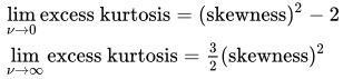
بدلاً من ذلك، يمكن التعبير عن التفرطح الزائد بدلالة المعلمتين التاليتين فقط: مربع الالتواء، وحجم العينة ν كما يلي:

من هذا التعبير الأخير، يمكن الحصول على نفس الحدود التي نشرها كارل بيرسون [ 21 ] منذ أكثر من قرن لتوزيع بيتا (انظر القسم أدناه بعنوان "التفرطح المحدود بمربع الالتواء"). بوضع α + β = ν = 0 في التعبير أعلاه، نحصل على الحد الأدنى لبيرسون (لا يمكن أن تحدث قيم الالتواء والتفرطح الزائد أسفل هذا الحد ( التفرطح الزائد + 2 - الالتواء 2 = 0) لأي توزيع، ولذلك أطلق كارل بيرسون على المنطقة الواقعة أسفل هذا الحد اسم "المنطقة المستحيلة"). تحدد نهاية α + β = ν → ∞ الحد الأعلى لبيرسون.
لذلك:

قيم ν = α + β بحيث تتراوح ν من الصفر إلى اللانهاية، 0 < ν < ∞، تغطي المنطقة بأكملها لتوزيع بيتا في مستوى التفرطح الزائد مقابل التواء المربع.
في الحالة المتناظرة ( α = β )، تنطبق الحدود التالية:
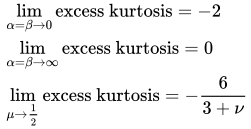
بالنسبة للحالات غير المتماثلة ( α ≠ β )، يمكن الحصول على النهايات التالية (مع اقتراب المتغير المذكور فقط من النهاية) من التعبيرات المذكورة أعلاه:


الدالة المميزة


الدالة المميزة هي تحويل فورييه لدالة كثافة الاحتمال. الدالة المميزة لتوزيع بيتا هي دالة كومر الهندسية الفائقة المتقاربة (من النوع الأول): [ 1 ] [ 18 ] [ 22 ]
- ;\beta ;t)&=\operatorname {E} \left[e^{itX}\right]\\&=\int _{0}^{1}e^{itx}f(x;\alpha ,\beta )\,dx\\&={}_{1}F_{1}(\alpha ;\alpha +\beta ;it)\!\\&=\sum _{n=0}^{\infty }{\frac {\alpha ^{\overline {n}}(it)^{n}}{(\alpha +\beta )^{\overline {n}}n!}}\\&=1+\sum _{k=1}^{\infty }\left(\prod _{r=0}^{k-1}{\frac {\alpha +r}{\alpha +\beta +r}}\right){\frac {(it)^{k}}{k!}}\end{aligned}}}
![\begin{aligned}\varphi_{X}(\alpha;\beta;t)&=\operatorname{E}\left[e^{itX}\right]\\&=\int_{0}^{1}e^{itx}f(x;\alpha,\beta)\,dx\\&={}_{1}F_{1}(\alpha;\alpha +\beta;it)\!\\&=\sum_{n=0}^{\infty}{\frac{\alpha^{\overline{n}}(it)^{n}}{(\alpha +\beta)^{\overline{n}}n!}}\\&=1+\sum_{k=1}^{\infty}\left(\prod_{r=0}^{k-1}{\frac{\alpha +r}{\alpha} +\beta +r}}\right){\frac {(it)^{k}}{k!}}\end{aligned}}}](https://wikimedia.org/api/rest_v1/media/math/render/svg/2e0e8f5d3bf4ec0cbe9b911e26c961e9ebaefdd8)
أين

هو المضروب المتزايد . قيمة الدالة المميزة عند t = 0 تساوي واحدًا:
;\beta ;0)={}_{1}F_{1}(\alpha ;\alpha +\beta ;0)=1.}

كذلك، تتمتع الأجزاء الحقيقية والخيالية للدالة المميزة بالتناظرات التالية بالنسبة لأصل المتغير t :
;\alpha +\beta ;it)\right]=\operatorname {Re} \left[{}_{1}F_{1}(\alpha ;\alpha +\beta ;-it)\right]} ;\alpha +\beta ;it)\right]=-\operatorname {Im} \left[{}_{1}F_{1}(\alpha ;\alpha +\beta ;-it)\right]}
![{\displaystyle \operatorname {Re} \left[{}_{1}F_{1}(\alpha ;\alpha +\beta ;it)\right]=\operatorname {Re} \left[{}_{1}F_{1}(\alpha ;\alpha +\beta ;-it)\right]}](https://wikimedia.org/api/rest_v1/media/math/render/svg/468f2135d76bd1b522c84092679209ff6abd5845)
![{\displaystyle \operatorname {Im} \left[{}_{1}F_{1}(\alpha ;\alpha +\beta ;it)\right]=-\operatorname {Im} \left[{}_{1}F_{1}(\alpha ;\alpha +\beta ;-it)\right]}](https://wikimedia.org/api/rest_v1/media/math/render/svg/0fca8984292cc85cb8a37ecb5a2b7c04b5596282)
تُبسط الحالة المتناظرة α = β الدالة المميزة لتوزيع بيتا إلى دالة بيسل ، لأنه في الحالة الخاصة α + β = 2α ، تختزل الدالة الهندسية الفائقة المتقاربة (من النوع الأول) إلى دالة بيسل (دالة بيسل المعدلة من النوع الأول ).) باستخدام تحويل كومر الثاني على النحو التالي:

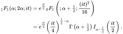
في الرسومات البيانية المصاحبة، يتم عرض الجزء الحقيقي (Re) من الدالة المميزة لتوزيع بيتا للحالات المتماثلة ( α = β ) والمنحرفة ( α ≠ β ).
لحظات أخرى
دالة توليد العزوم
ويترتب على ذلك أيضًا [ 1 ] [ 9 ] أن دالة توليد العزوم هي
;\beta ;t)&=\operatorname {E} \left[e^{tX}\right]\\[4pt]&=\int _{0}^{1}e^{tx}f(x;\alpha ,\beta )\,dx\\[4pt]&={}_{1}F_{1}(\alpha ;\alpha +\beta ;t)\\[4pt]&=\sum _{n=0}^{\infty }{\frac {\alpha ^{\overline {n}}}{(\alpha +\beta )^{\overline {n}}}}{\frac {t^{n}}{n!}}\\[4pt]&=1+\sum _{k=1}^{\infty }\left(\prod _{r=0}^{k-1}{\frac {\alpha +r}{\alpha +\beta +r}}\right){\frac {t^{k}}{k!}}.\end{aligned}}}
![{\displaystyle {\begin{aligned}M_{X}(\alpha ;\beta ;t)&=\operatorname {E} \left[e^{tX}\right]\\[4pt]&=\int _{0}^{1}e^{tx}f(x;\alpha ,\beta )\,dx\\[4pt]&={}_{1}F_{1}(\alpha ;\alpha +\beta ;t)\\[4pt]&=\sum _{n=0}^{\infty }{\frac {\alpha ^{\overline {n}}}{(\alpha +\beta )^{\overline {n}}}}{\frac {t^{n}}{n!}}\\[4pt]&=1+\sum _{k=1}^{\infty }\left(\prod _{r=0}^{k-1}{\frac {\alpha +r}{\alpha +\beta +r}}\right){\frac {t^{k}}{k!}}.\end{aligned}}}](https://wikimedia.org/api/rest_v1/media/math/render/svg/7c5c0eea7bcffadb73fef0c85534a8bdca36ebbb)
على وجه الخصوص M X ( α ; β ; 0) = 1.
لحظات أسمى
باستخدام دالة توليد العزوم ، يُعطى العزم الخام رقم k بالعامل [ 1 ]
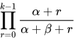
ضرب الحد (المتسلسلة الأسية)في سلسلة دالة توليد العزوم

![{\displaystyle \operatorname {E} [X^{k}]={\frac {\alpha ^{\overline {k}}}{(\alpha +\beta )^{\overline {k}}}}=\prod _{r=0}^{k-1}{\frac {\alpha +r}{\alpha +\beta +r}}}](https://wikimedia.org/api/rest_v1/media/math/render/svg/af7e0927f7f82eccc61e9fb55883ce96d7f958f1)
حيث يمثل ( x ) ( k ) رمز بوخامر الذي يمثل المضروب المتزايد. ويمكن كتابته أيضًا بصيغة تكرارية كما يلي:
![{\displaystyle \operatorname {E} [X^{k}]={\frac {\alpha +k-1}{\alpha +\beta +k-1}}\operatorname {E} [X^{k-1}].}](https://wikimedia.org/api/rest_v1/media/math/render/svg/069cb373a905b1e8a5a82a0e3b028e88f63672e2)
منذ لحظة توليد الدالة ;\beta ;\cdot )} له نصف قطر تقارب موجب،ويتم تحديد توزيع بيتا بواسطة لحظاته . [ 23 ]

لحظات المتغيرات العشوائية المحولة
لحظات المتغيرات العشوائية المحولة خطيًا، والمُنتَجة، والمعكوسة
يمكن أيضًا إظهار التوقعات التالية لمتغير عشوائي مُحوَّل، [ 1 ] حيث يكون المتغير العشوائي X مُوزَّعًا وفقًا لتوزيع بيتا بمعاملات α و β : X ~ Beta( α , β ). القيمة المتوقعة للمتغير 1 − X هي انعكاس القيمة المتوقعة بناءً على X.
![\begin{aligned}\operatorname {E} [1-X]&={\frac {\beta }{\alpha +\beta }}\\\operatorname {E} [X(1-X)]&=\operatorname {E} [(1-X)X]={\frac {\alpha \beta }{(\alpha +\beta )(\alpha +\beta +1)}}\end{aligned}}}](https://wikimedia.org/api/rest_v1/media/math/render/svg/43fc49b9eafccd56d39c236b26d222dde51638ce)
بسبب التناظر المرآوي لدالة كثافة الاحتمال لتوزيع بيتا، فإن التباينات المستندة إلى المتغيرات X و 1 − X متطابقة، والتباين المشترك على X (1 − X ) هو معكوس التباين:
![{\displaystyle \operatorname {var} [(1-X)]=\operatorname {var} [X]=-\operatorname {cov} [X,(1-X)]={\frac {\alpha \beta }{(\alpha +\beta )^{2}(\alpha +\beta +1)}}}](https://wikimedia.org/api/rest_v1/media/math/render/svg/7273cc84a6c789724b985c34059fa75a62bce631)
هذه هي القيم المتوقعة للمتغيرات المعكوسة (وهي مرتبطة بالمتوسطات التوافقية، انظر § المتوسط التوافقي ):
![\begin{aligned}\operatorname {E} \left[{\frac {1}{X}}\right]&={\frac {\alpha +\beta -1}{\alpha -1}}&&{\text{ إذا كان }}\alpha >1\\\operatorname {E} \left[{\frac {1}{1-X}}\right]&={\frac {\alpha +\beta -1}{\beta -1}}&&{\text{ إذا كان }}\beta >1\end{aligned}}}](https://wikimedia.org/api/rest_v1/media/math/render/svg/972a9c1853e6991aac6666b06c0a633a0caad5b7)
ينتج عن التحويل التالي بقسمة المتغير X على صورته المرآوية X /(1 − X )) القيمة المتوقعة لـ "توزيع بيتا المعكوس" أو توزيع بيتا الأولي (المعروف أيضًا باسم توزيع بيتا من النوع الثاني أو النوع السادس لبيرسون ): [ 1 ]
![\begin{aligned}\operatorname {E} \left[{\frac {X}{1-X}}\right]&={\frac {\alpha }{\beta -1}}&&{\text{ إذا كان }}\beta >1\\\operatorname {E} \left[{\frac {1-X}{X}}\right]&={\frac {\beta }{\alpha -1}}&&{\text{ إذا كان }}\alpha >1\end{aligned}}}](https://wikimedia.org/api/rest_v1/media/math/render/svg/db2a0928a7f906bcbe5cfd9d0c57713c9ab5cfb7)
يمكن الحصول على تباينات هذه المتغيرات المحولة عن طريق التكامل، باعتبارها القيم المتوقعة للعزوم الثانية المتمركزة حول المتغيرات المقابلة:
![\displaystyle \begin{aligned}\operatorname {var} \left[{\frac {1}{X}}\right]&=\operatorname {E} \left[\left({\frac {1}{X}}-\operatorname {E} \left[{\frac {1}{X}}\right]\right)^{2}\right]=\operatorname {var} \left[{\frac {1-X}{X}}\right]\\&=\operatorname {E} \left[\left({\frac {1-X}{X}}-\operatorname {E} \left[{\frac {1-X}{X}}\right]\right)^{2}\right]={\frac {\beta (\alpha +\beta -1)}{\left(\alpha -2\right)\left(\alpha -1)^{2}}{\text{ إذا }}\alpha >2\end{aligned}}}](https://wikimedia.org/api/rest_v1/media/math/render/svg/ab8c3db5d04798c92c6360624060ba583ebdf3df)
ينتج عن التباين التالي للمتغير X مقسومًا على صورته المرآوية ( X /(1− X ) تباين "توزيع بيتا المعكوس" أو توزيع بيتا الأولي (المعروف أيضًا باسم توزيع بيتا من النوع الثاني أو النوع السادس لبيرسون ): [ 1 ]
![\displaystyle \begin{aligned}\operatorname {var} \left[{\frac {1}{1-X}}\right]&=\operatorname {E} \left[\left({\frac {1}{1-X}}-\operatorname {E} \left[{\frac {1}{1-X}}\right]\right)^{2}\right]=\operatorname {var} \left[{\frac {X}{1-X}}\right]\\[1ex]&=\operatorname {E} \left[\left({\frac {X}{1-X}}-\operatorname {E} \left[{\frac {X}{1-X}}\right]\right)^{2}\right]={\frac {\alpha (\alpha +\beta -1)}{\left(\beta -2\right)\left(\beta -1)^{2}}}{\text{ إذا }}\beta >2\end{aligned}}}](https://wikimedia.org/api/rest_v1/media/math/render/svg/76d83000746ff4852e63b063948f9db8110d2d22)
التغايرات هي:
تظهر هذه التوقعات والتباينات في مصفوفة معلومات فيشر ذات المعلمات الأربع ( § معلومات فيشر .)
![{\displaystyle {\begin{aligned}\operatorname {cov} \left[{\frac {1}{X}},{\frac {1}{1-X}}\right]&=\operatorname {cov} \left[{\frac {1-X}{X}},{\frac {X}{1-X}}\right]=\operatorname {cov} \left[{\frac {1}{X}},{\frac {X}{1-X}}\right]\\[1ex]&=\operatorname {cov} \left[{\frac {1-X}{X}},{\frac {1}{1-X}}\right]={\frac {\alpha +\beta -1}{(\alpha -1)(\beta -1)}}{\text{ إذا كان }}\alpha ,\beta >1\end{aligned}}}](https://wikimedia.org/api/rest_v1/media/math/render/svg/ce6ebb40e9f206c0269353799307092c2edbcfa0)
لحظات المتغيرات العشوائية المحولة لوغاريتميًا
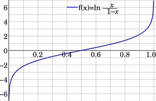
تُناقش في هذا القسم القيم المتوقعة للتحويلات اللوغاريتمية (المفيدة لتقديرات الاحتمال الأقصى ، انظر § تقدير المعلمات، الاحتمال الأقصى ). وترتبط التحويلات الخطية اللوغاريتمية التالية بالمتوسطات الهندسية G( X) و G (1- X) (انظر § المتوسط الهندسي ):
![\displaystyle \begin{aligned}\operatorname {E} [\ln X]&=\psi (\alpha )-\psi (\alpha +\beta )=-\operatorname {E} \left[\ln {\frac {1}{X}}\right],\\\operatorname {E} [\ln(1-X)]&=\psi (\beta )-\psi (\alpha +\beta )=-\operatorname {E} \left[\ln {\frac {1}{1-X}}\right].\end{aligned}}}](https://wikimedia.org/api/rest_v1/media/math/render/svg/af6c3188ac96160054472db2a23bab9a22f1e486)
حيث يتم تعريف دالة ديجاما ψ ( α ) على أنها المشتق اللوغاريتمي لدالة جاما : [ 18 ]

تُعد تحويلات اللوجيت مثيرة للاهتمام، [ 24 ] لأنها عادةً ما تحول الأشكال المختلفة (بما في ذلك الأشكال J) إلى كثافات على شكل جرس (عادةً ما تكون منحرفة) على متغير اللوجيت، وقد تزيل النقاط الشاذة النهائية على المتغير الأصلي:
![\displaystyle \begin{aligned}\operatorname {E} \left[\ln {\frac {X}{1-X}}\right]&=\psi (\alpha )-\psi (\beta )=\operatorname {E} [\ln X]+\operatorname {E} \left[\ln {\frac {1}{1-X}}\right],\\\operatorname {E} \left[\ln {\frac {1-X}{X}}\right]&=\psi (\beta )-\psi (\alpha )=-\operatorname {E} \left[\ln {\frac {X}{1-X}}\right].\end{aligned}}}](https://wikimedia.org/api/rest_v1/media/math/render/svg/a30b0fbbefff93de41d6775f2ab623670f09a4b2)
درس جونسون [ 25 ] توزيع المتغير المحوّل لوجيت ln( X /1 − X )، بما في ذلك دالة توليد العزوم والتقريبات للقيم الكبيرة لمعاملات الشكل. يُوسّع هذا التحويل المجال المحدود [0, 1] القائم على المتغير الأصلي X إلى مجال غير محدود في كلا اتجاهي خط الأعداد الحقيقية (−∞, +∞). يتبع لوجيت متغير بيتا توزيع لوجستي-بيتا .
يمكن اشتقاق العزوم اللوغاريتمية من الرتب العليا باستخدام تمثيل توزيع بيتا كنسبة من توزيعين غاما، ثم اشتقاق التكامل. ويمكن التعبير عنها بدلالة دوال غاما المتعددة من الرتب العليا كما يلي:
![\begin{aligned}\operatorname {E} \left[\ln ^{2}(X)\right]&=(\psi (\alpha )-\psi (\alpha +\beta ))^{2}+\psi _{1}(\alpha )-\psi _{1}(\alpha +\beta ),\\\operatorname {E} \left[\ln ^{2}(1-X)\right]&=(\psi (\beta )-\psi (\alpha +\beta ))^{2}+\psi _{1}(\beta )-\psi _{1}(\alpha +\beta ),\\\operatorname {E} \left[\ln(X)\ln(1-X)\right]&=(\psi (\alpha )-\psi (\alpha +\beta ))(\psi (\beta )-\psi (\alpha +\beta ))-\psi _{1}(\alpha +\beta ).\end{aligned}}}](https://wikimedia.org/api/rest_v1/media/math/render/svg/b42eb1276e349df39df3051df11e0e16afe88e2e)
وبالتالي فإن تباين المتغيرات اللوغاريتمية والتباين المشترك لـ ln( X ) و ln(1− X ) هما:
![\displaystyle \begin{aligned}\operatorname {cov} [\ln X,\ln(1-X)]&=\operatorname {E} \left[\ln X\ln(1-X)\right]-\operatorname {E} [\ln X]\operatorname {E} [\ln(1-X)]\\&=-\psi _{1}(\alpha +\beta )\\&\\\operatorname {var} [\ln X]&=\operatorname {E} [\ln ^{2}X]-(\operatorname {E} [\ln X])^{2}\\&=\psi _{1}(\alpha )-\psi _{1}(\alpha +\beta )\\&=\psi _{1}(\alpha )+\operatorname {cov} [\ln X,\ln(1-X)]\\&\\\operatorname {var} [\ln(1-X)]&=\operatorname {E} [\ln ^{2}(1-X)]-(\operatorname {E} [\ln(1-X)])^{2}\\&=\psi _{1}(\beta )-\psi _{1}(\alpha +\beta )\\&=\psi _{1}(\beta )+\operatorname {cov} [\ln X,\ln(1-X)]\end{aligned}}}](https://wikimedia.org/api/rest_v1/media/math/render/svg/53f5f8222528ab3aa1e5f610f49d440d348f7d40)
حيث أن دالة تريغاما ، التي يرمز لها بـ ψ 1 ( α )، هي الثانية من دوال بوليغاما ، وتُعرف بأنها مشتقة دالة ديغاما :
إن التباينات والتباين المشترك للمتغيرات المحولة لوغاريتميًا X و (1 − X ) مختلفة بشكل عام، لأن التحويل اللوغاريتمي يدمر التناظر المرآوي للمتغيرات الأصلية X و (1 − X )، حيث يقترب اللوغاريتم من اللانهاية السالبة للمتغير الذي يقترب من الصفر.
تُعدّ هذه التباينات والتباينات المشتركة اللوغاريتمية عناصر مصفوفة معلومات فيشر لتوزيع بيتا. كما أنها تُشكّل مقياسًا لانحناء دالة الاحتمال اللوغاريتمي (انظر قسم تقدير الاحتمال الأقصى).
إن تباينات معكوس اللوغاريتمات متطابقة مع تباينات اللوغاريتمات:
![\begin{aligned}\operatorname{var} \left[\ln{\frac{1}{X}}\right]&=\operatorname{var}[\lnX]=\psi_{1}(\alpha)-\psi_{1}(\alpha +\beta),\\\operatorname{var} \left[\ln{\frac{1}{1-X}}\right]&=\operatorname{var}[\ln(1-X)]=\psi_{1}(\beta)-\psi_{1}(\alpha +\beta),\\\operatorname{cov} \left[\ln{\frac{1}{X}},\,\ln{\frac{1}{1-X}}\right]&=\operatorname{cov}[\lnX,\ln(1-X)]=-\psi _{1}(\alpha +\beta ).\end{aligned}}}](https://wikimedia.org/api/rest_v1/media/math/render/svg/18739db82ac6e431571537bb8f09ff006d670b04)
ويترتب على ذلك أيضاً أن تباينات المتغيرات المحولة باستخدام دالة اللوجيت هي
![\begin{aligned}\operatorname{var} \left[\ln{\frac{X}{1-X}}\right]&=\operatorname{var} \left[\ln{\frac{1-X}{X}}\right]\\&=-\operatorname{cov} \left[\ln{\frac{X}{1-X}},\,\ln{\frac{1-X}{X}}\right]\\[1ex]&=\psi_{1}(\alpha)+\psi_{1}(\beta).\end{aligned}}}](https://wikimedia.org/api/rest_v1/media/math/render/svg/b0f473b85a33bfd20c16bd2e752af80def37388a)
كميات المعلومات (الإنتروبيا)
بالنظر إلى متغير عشوائي موزع بيتا، X ~ Beta( α , β )، فإن الإنتروبيا التفاضلية لـ X هي (مقاسة بالنات )، [ 26 ] القيمة المتوقعة لسالب لوغاريتم دالة كثافة الاحتمال :
![{\displaystyle {\begin{aligned}h(X)&=\operatorname {E} \left[-\ln f(X;\alpha ,\beta )\right]\\[4pt]&=\int _{0}^{1}-f(x;\alpha ,\beta )\ln f(x;\alpha ,\beta )\,dx\\[4pt]&=\ln \mathrm {B} (\alpha ,\beta )-(\alpha -1)\psi (\alpha )-(\beta -1)\psi (\beta )+(\alpha +\beta -2)\psi (\alpha +\beta )\end{aligned}}}](https://wikimedia.org/api/rest_v1/media/math/render/svg/ee7535c40811773d4239dc63ea6c2200c4b7a63c)
حيث f ( x ; α , β ) هي دالة كثافة الاحتمال لتوزيع بيتا:

تظهر دالة ديغاما ψ في صيغة الإنتروبيا التفاضلية كنتيجة لصيغة أويلر التكاملية للأعداد التوافقية التي تتبع من التكامل:

تكون الإنتروبيا التفاضلية لتوزيع بيتا سالبة لجميع قيم α و β الأكبر من الصفر، باستثناء α = β = 1 (حيث يكون توزيع بيتا هو نفسه التوزيع المنتظم )، إذ تصل الإنتروبيا التفاضلية إلى قيمتها القصوى وهي الصفر. ومن المتوقع أن تحدث الإنتروبيا القصوى عندما يصبح توزيع بيتا مساويًا للتوزيع المنتظم، لأن عدم اليقين يكون في أقصى حالاته عندما تكون جميع الأحداث المحتملة متساوية الاحتمال.
عندما تقترب قيمة α أو β من الصفر، تقترب الإنتروبيا التفاضلية من قيمتها الدنيا وهي سالب ما لا نهاية. وعندما تقترب قيمة α أو β (أو كلتاهما) من الصفر، يكون هناك أقصى قدر من الترتيب: تتركز كثافة الاحتمال بالكامل عند الأطراف، وتكون كثافة الاحتمال صفرًا عند النقاط الواقعة بين الأطراف. وبالمثل، عندما تقترب قيمة α أو β (أو كلتاهما) من اللانهاية، تقترب الإنتروبيا التفاضلية من قيمتها الدنيا وهي سالب ما لا نهاية، ويكون هناك أقصى قدر من الترتيب. إذا اقتربت قيمة α أو β من اللانهاية (وكانت الأخرى محدودة)، تتركز كثافة الاحتمال بالكامل عند أحد الأطراف، وتكون كثافة الاحتمال صفرًا في أي مكان آخر. إذا كان كلا معاملي الشكل متساويين (الحالة المتناظرة)، α = β ، واقتربا من اللانهاية في الوقت نفسه، تصبح كثافة الاحتمال على شكل قمة حادة ( دالة ديراك دلتا ) تتركز عند المنتصف x = 1/2، وبالتالي يكون الاحتمال 100% عند المنتصف x = 1/2، ويكون الاحتمال صفرًا في أي مكان آخر.


قدّم شانون مفهوم الإنتروبيا التفاضلية (في الحالة المستمرة) في بحثه الأصلي (حيث أطلق عليها اسم "إنتروبيا التوزيع المستمر")، كجزء ختامي من البحث نفسه الذي عرّف فيه الإنتروبيا المتقطعة . [ 27 ] ومنذ ذلك الحين، بات معروفًا أن الإنتروبيا التفاضلية قد تختلف عن الحد المتناهي الصغر للإنتروبيا المتقطعة بمقدار لانهائي، وبالتالي يمكن أن تكون الإنتروبيا التفاضلية سالبة (كما هو الحال في توزيع بيتا). لكن الأهم هو القيمة النسبية للإنتروبيا.
بالنظر إلى متغيرين عشوائيين موزعين بيتا، X 1 ~ Beta( α , β ) و X 2 ~ Beta( α ′ , β ′ )، فإن الإنتروبيا المتقاطعة هي (مقاسة بالنات) [ 28 ].
![{\displaystyle {\begin{aligned}H(X_{1},X_{2})&=\int _{0}^{1}-f(x;\alpha ,\beta )\ln f(x;\alpha ',\beta ')\,dx\\[4pt]&=\ln \mathrm {B} (\alpha ',\beta ')-(\alpha '-1)\psi (\alpha )-(\beta '-1)\psi (\beta )+\left(\alpha '+\beta '-2\right)\psi (\alpha +\beta ).\end{aligned}}}](https://wikimedia.org/api/rest_v1/media/math/render/svg/f9e7662d68f802bd6e6b1019f0eb46e6a4bfc0a4)
استُخدمت الإنتروبيا المتقاطعة كمقياس للخطأ لقياس المسافة بين فرضيتين. [ 29 ] [ 30 ] وتكون قيمتها المطلقة في أدنى مستوياتها عندما يكون التوزيعان متطابقين. وهي مقياس المعلومات الأكثر ارتباطًا باللوغاريتم الأقصى للاحتمالية [ 28 ] (انظر القسم الخاص بـ "تقدير المعلمات. تقدير الاحتمالية القصوى").
الإنتروبيا النسبية، أو تباعد كولباك-لايبير D KL ( X 1 || X 2 )، هي مقياس لعدم كفاءة افتراض أن التوزيع X 2 ~ Beta( α ′ , β ′ ) عندما يكون التوزيع في الواقع X 1 ~ Beta( α , β ). ويتم تعريفها كما يلي (مقاسة بالناتس).
![{\displaystyle {\begin{aligned}D_{\mathrm {KL} }(X_{1}\parallel X_{2})&=\int _{0}^{1}f(x;\alpha ,\beta )\,\ln {\frac {f(x;\alpha ,\beta )}{f(x;\alpha ',\beta ')}}\,dx\\[4pt]&=\left(\int _{0}^{1}f(x;\alpha ,\beta )\ln f(x;\alpha ,\beta )\,dx\right)-\left(\int _{0}^{1}f(x;\alpha ,\beta )\ln f(x;\alpha ',\beta ')\,dx\right)\\[4pt]&=-h(X_{1})+H(X_{1},X_{2})\\[4pt]&=\ln {\frac {\mathrm {B} (\alpha ',\beta ')}{\mathrm {B} (\alpha ,\beta )}}+\left(\alpha -\alpha '\right)\psi (\alpha )+\left(\beta -\beta '\right)\psi (\beta )+\left(\alpha '-\alpha +\beta '-\beta \right)\psi (\alpha +\beta ).\end{aligned}}}](https://wikimedia.org/api/rest_v1/media/math/render/svg/533f00a1d061ebd96a170013f1339d34fc8f1322)
تكون الإنتروبيا النسبية، أو تباعد كولباك-لايبير ، دائمًا غير سالبة. وفيما يلي بعض الأمثلة العددية:
- X1 ~ Beta(1, 1) و X2 ~ Beta (3, 3)؛ D KL ( X1 || X2 ) = 0.598803؛ D KL ( X2 || X1 ) = 0.267864؛ h ( X1 ) = 0؛ h ( X2 ) = −0.267864
- X 1 ~ Beta(3, 0.5) و X 2 ~ Beta(0.5, 3)؛ D KL ( X 1 || X 2 ) = 7.21574؛ D KL ( X 2 || X 1 ) = 7.21574؛ h ( X 1 ) = −1.10805؛ h ( X 2 ) = −1.10805.
لا يكون تباعد كولباك-لايبير متناظرًا ( DKL ( X1 || X2 ) ≠ DKL ( X2 || X1 ) ) في حالة كون توزيعات بيتا الفردية Beta ( 1,1 ) وBeta(3,3) متناظرة، ولكن لها إنتروبيا مختلفة ( h ( X1 ) ≠ h ( X2 ) ). تعتمد قيمة تباعد كولباك على اتجاه التغير: سواء كان من إنتروبيا تفاضلية أعلى إلى إنتروبيا تفاضلية أقل ، أو العكس. في المثال العددي أعلاه، يقيس تباعد كولباك عدم كفاءة افتراض أن التوزيع هو Beta(3,3) (على شكل جرس)، بدلًا من Beta(1,1) (منتظم). تكون إنتروبيا "h" لتوزيع بيتا(1, 1) أعلى من إنتروبيا "h" لتوزيع بيتا(3, 3) لأن التوزيع المنتظم بيتا(1, 1) يتميز بأقصى قدر من الفوضى. ويكون تباعد كولباك أعلى بأكثر من الضعف (0.598803 بدلاً من 0.267864) عند قياسه في اتجاه تناقص الإنتروبيا: وهو الاتجاه الذي يفترض أن توزيع بيتا(1, 1) (المنتظم) هو توزيع بيتا(3, 3) (على شكل جرس) وليس العكس. وبهذا المعنى المحدد، يتوافق تباعد كولباك مع القانون الثاني للديناميكا الحرارية .
إن تباعد كولباك -لايبير متناظر D KL ( X 1 || X 2 ) = D KL ( X 2 || X 1 ) للحالات المنحرفة Beta(3, 0.5) و Beta(0.5, 3) التي لها إنتروبيا تفاضلية متساوية h ( X 1 ) = h ( X 2 ).
شرط التناظر:

ويتبع ذلك من التعريفات المذكورة أعلاه والتناظر المرآوي f ( x ; α , β ) = f (1 − x ; α , β ) الذي يتمتع به توزيع بيتا.
العلاقات بين المقاييس الإحصائية
العلاقة بين المتوسط والمنوال والوسيط
إذا كان 1 < α < β فإن المنوال ≤ الوسيط ≤ المتوسط. [ 10 ] التعبير عن المنوال (فقط عندما α و β > 1)، والمتوسط بدلالة α و β :

إذا كان 1 < β < α، فإن ترتيب المتباينات ينعكس. بالنسبة لـ α و β > 1، تكون المسافة المطلقة بين المتوسط والوسيط أقل من 5% من المسافة بين القيمتين العظمى والصغرى لـ x . من ناحية أخرى، قد تصل المسافة المطلقة بين المتوسط والمنوال إلى 50% من المسافة بين القيمتين العظمى والصغرى لـ x ، وذلك في الحالة الشاذة α = 1 و β = 1، حيث تقترب قيمة توزيع بيتا من التوزيع المنتظم، ويقترب الانتروبيا التفاضلي من قيمته القصوى ، وبالتالي يصل إلى أقصى درجات "الاضطراب".
على سبيل المثال، بالنسبة لـ α = 1.0001 و β = 1.00000001:
- المنوال = 0.9999؛ دالة كثافة الاحتمال (المنوال) = 1.00010
- المتوسط = 0.500025؛ دالة كثافة الاحتمال (المتوسط) = 1.00003
- الوسيط = 0.500035؛ دالة كثافة الاحتمال (الوسيط) = 1.00003
- المتوسط - المنوال = -0.499875
- المتوسط - الوسيط = -9.65538 × 10⁻⁶
حيث يرمز PDF إلى قيمة دالة كثافة الاحتمال .


العلاقة بين المتوسط، والمتوسط الهندسي، والمتوسط التوافقي

من المعروف من متباينة المتوسط الحسابي والمتوسط الهندسي أن المتوسط الهندسي أقل من المتوسط الحسابي. وبالمثل، فإن المتوسط التوافقي أقل من المتوسط الهندسي. يوضح الرسم البياني المرفق أنه عندما α = β ، يكون كل من المتوسط والوسيط مساويين تمامًا لـ 1/2، بغض النظر عن قيمة α = β ، ويكون المنوال مساويًا أيضًا لـ 1/2 عندما α = β > 1. مع ذلك، فإن المتوسطين الهندسي والتوافقي أقل من 1/2، ولا يقتربان من هذه القيمة إلا تقاربًا عندما α = β → ∞.
التفرطح محصور بمربع معامل الالتواء

كما أشار فيلر [ 5 ] ، في نظام بيرسون، يظهر توزيع بيتا الاحتمالي من النوع الأول (أي اختلاف بين توزيع بيتا وتوزيع بيرسون من النوع الأول هو اختلاف سطحي فقط، ولا يؤثر على المناقشة التالية المتعلقة بالعلاقة بين التفرطح والالتواء). عرض كارل بيرسون ، في اللوحة 1 من بحثه [ 21 ] المنشور عام 1916، رسمًا بيانيًا يمثل فيه التفرطح المحور الرأسي ( المحور الصادي ) ومربع الالتواء المحور الأفقي ( المحور السيني )، حيث عُرضت فيه عدة توزيعات. [ 31 ] المنطقة التي يشغلها توزيع بيتا محصورة بين الخطين التاليين في مستوى (الالتواء 2 ، التفرطح) ، أو مستوى (الالتواء 2 ، التفرطح الزائد) :

أو، على نحو مماثل،

في زمنٍ لم تكن فيه الحواسيب الرقمية القوية متوفرة، قام كارل بيرسون بحساب حدودٍ إضافية بدقة، [ 32 ] [ 21 ] على سبيل المثال، فصل التوزيعات "على شكل حرف U" عن التوزيعات "على شكل حرف J". ينتج خط الحد السفلي (التفرطح الزائد + 2 - معامل الالتواء 2 = 0) عن توزيعات بيتا "على شكل حرف U" ملتوية، حيث تكون قيم معاملي الشكل α و β قريبة من الصفر. أما خط الحد العلوي (التفرطح الزائد - (3/2) معامل الالتواء 2 = 0) فينتج عن توزيعات شديدة الالتواء، حيث تكون قيم أحد المعاملين كبيرة جدًا، وقيم المعامل الآخر صغيرة جدًا. أظهر كارل بيرسون [ 21 ] أن خط الحد العلوي هذا (التفرطح الزائد - مربع الالتواء (3/2) = 0) هو أيضًا نقطة تقاطع مع توزيع بيرسون من النوع الثالث، والذي له نطاق غير محدود في اتجاه واحد (نحو اللانهاية الموجبة)، ويمكن أن يكون على شكل جرس أو على شكل حرف J. وأظهر ابنه، إيغون بيرسون [ 31 ] أن المنطقة (في مستوى التفرطح/مربع الالتواء) التي يشغلها توزيع بيتا (أو توزيع بيرسون من النوع الأول) عند اقترابه من هذا الحد (التفرطح الزائد - مربع الالتواء (3/2) = 0) مشتركة مع توزيع كاي تربيع غير المركزي . كما أظهر كارل بيرسون [ 33 ] (بيرسون 1895، الصفحات 357، 360، 373-376) أن توزيع غاما هو توزيع من النوع الثالث لبيرسون. لذا، يُعرف هذا الخط الحدودي لتوزيع بيرسون من النوع الثالث بخط غاما. (يتضح ذلك من حقيقة أن التفرطح الزائد لتوزيع غاما يساوي 6/ k ، ومربع الالتواء يساوي 4/ k ، وبالتالي فإن المعادلة (التفرطح الزائد - (3/2) الالتواء² = 0) تتحقق بشكل مطابق في توزيع غاما بغض النظر عن قيمة المعامل "k"). لاحقًا، لاحظ بيرسون أن توزيع كاي تربيع هو حالة خاصة من توزيع بيرسون من النوع الثالث، ويشترك أيضًا في هذا الخط الحدودي (كما يتضح من حقيقة أن التفرطح الزائد لتوزيع كاي تربيع يساوي 12/ k، ومربع الالتواء يساوي 8/ k ، وبالتالي فإن المعادلة (التفرطح الزائد - (3/2) الالتواء² = 0) تتحقق بشكل مطابق بغض النظر عن قيمة المعامل "k"). وهذا أمر متوقع، لأن توزيع كاي تربيع X ~ χ² ( k )) هي حالة خاصة من توزيع جاما، مع المعلمة X ~ Γ(k/2, 1/2) حيث k هو عدد صحيح موجب يحدد "عدد درجات الحرية" لتوزيع مربع كاي.
مثال على توزيع بيتا بالقرب من الحد الأعلى (التفرطح الزائد - (3/2) معامل الالتواء 2 = 0) يُعطى بالعلاقة α = 0.1، β = 1000، حيث تقترب النسبة (التفرطح الزائد)/(معامل الالتواء 2 ) = 1.49835 من الحد الأعلى 1.5 من الأسفل. مثال على توزيع بيتا بالقرب من الحد الأدنى (التفرطح الزائد + 2 - معامل الالتواء 2 = 0) يُعطى بالعلاقة α = 0.0001، β = 0.1، حيث تقترب النسبة (التفرطح الزائد + 2)/(معامل الالتواء 2 ) = 1.01621 من الحد الأدنى 1 من الأعلى. في حالة التقارب المتناهي الصغر، عندما تقترب كل من α و β من الصفر بشكل متناظر، يصل التفرطح الزائد إلى أدنى قيمة له عند -2. تحدث هذه القيمة الدنيا عند النقطة التي يتقاطع فيها خط الحد السفلي مع المحور الرأسي ( المحور الإحداثي ). (مع ذلك، في مخطط بيرسون الأصلي، يمثل المحور الإحداثي التفرطح، بدلاً من التفرطح الزائد، ويزداد باتجاه الأسفل بدلاً من الأعلى).
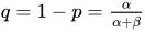
لا يمكن أن تحدث قيم الالتواء والتفرطح الزائد دون الحد الأدنى (التفرطح الزائد + 2 - الالتواء 2 = 0) لأي توزيع، ولذلك أطلق كارل بيرسون على المنطقة الواقعة أسفل هذا الحد اسم "المنطقة المستحيلة". يُحدد حد هذه "المنطقة المستحيلة" بواسطة توزيعات ثنائية النمط على شكل حرف U (متماثلة أو ملتوية) حيث تقترب المعلمتان α و β من الصفر، وبالتالي تتركز كثافة الاحتمال عند الطرفين: x = 0 و 1، مع انعدام القيم عمليًا بينهما. وبما أن كثافة الاحتمال تتركز عند الطرفين x = 0 و x = 1 عندما α ≈ β ≈ 0 ، فإن هذا "الحد المستحيل" يُحدد بواسطة توزيع برنولي ، حيث لا توجد سوى نتيجتين ممكنتين باحتمالين p و q = 1 - p على التوالي . في الحالات التي تقترب من هذا الحدّ مع التناظر α = β ، يكون معامل الالتواء ≈ 0، ومعامل التفرطح الزائد ≈ −2 (وهو أدنى معامل تفرطح زائد ممكن لأي توزيع)، وتكون الاحتمالات p ≈ q ≈ 1/2. أما في الحالات التي تقترب من هذا الحدّ مع معامل الالتواء، ومعامل التفرطح الزائد ≈ −2 + معامل الالتواء 2 ، ويكون تركيز دالة الاحتمال أكبر عند أحد طرفي التوزيع مقارنةً بالطرف الآخر (مع انعدام القيم تقريبًا بينهما)، فتكون الاحتمالات عند الطرف الأيسر x = 0 وعند الطرف الأيمن x = 1.

التناظر
جميع العبارات مشروطة بـ α و β > 0:
- تناظر انعكاس دالة كثافة الاحتمال
- دالة التوزيع التراكمي ، تناظر الانعكاس، بالإضافة إلى التحويل الوحدوي
- نمط التناظر الانعكاسي بالإضافة إلى الإزاحة الوحدوية
- تناظر الانعكاس المتوسط بالإضافة إلى الإزاحة الوحدوية
- تناظر الانعكاس المتوسط بالإضافة إلى الإزاحة الوحدوية
- يعني مصطلح "هندسي" أن كل عنصر غير متماثل على حدة، وينطبق التناظر التالي بين المتوسط الهندسي القائم على X والمتوسط الهندسي القائم على انعكاسه 1− X
- يعني مصطلح "توافقي" أن كل عنصر غير متماثل بشكل فردي، وينطبق التناظر التالي بين المتوسط التوافقي القائم على X والمتوسط التوافقي القائم على انعكاسه 1− X
- تناظر التباين
- كل تباين هندسي غير متماثل على حدة، وينطبق التناظر التالي بين التباين الهندسي اللوغاريتمي القائم على X والتباين الهندسي اللوغاريتمي القائم على انعكاسه 1− X
- التناظر الهندسي المتباين
- متوسط الانحراف المطلق حول التناظر المتوسط
- التواء التناظر
- تناظر التفرطح الزائد
- تناظر الدالة المميزة للجزء الحقيقي (بالنسبة لأصل المتغير " t ") ;\alpha +\beta ;it)]={\text{Re}}[{}_{1}F_{1}(\alpha ;\alpha +\beta ;-it)]}
- التناظر المعكوس للدالة المميزة للجزء التخيلي (بالنسبة لأصل المتغير " t ") ;\alpha +\beta ;it)]=-{\text{Im}}[{}_{1}F_{1}(\alpha ;\alpha +\beta ;-it)]}
- تناظر الدالة المميزة للقيمة المطلقة (بالنسبة لأصل المتغير " t ") ;\alpha +\beta ;it)]={\text{Abs}}[{}_{1}F_{1}(\alpha ;\alpha +\beta ;-it)]}
- تناظر الإنتروبيا التفاضلية
- تناظر الإنتروبيا النسبية (يسمى أيضًا تباعد كولباك-لايبير )
- تناظر مصفوفة معلومات فيشر








![{\displaystyle \operatorname {E} [|XE[X]|](\mathrm {B} (\alpha ,\beta )=\operatorname {E} [|XE[X]|](\mathrm {B} (\beta ,\alpha ))}](https://wikimedia.org/api/rest_v1/media/math/render/svg/83468b7365d9095b07e04bfbb5c9cff50c64ea2d)


![{\displaystyle {\text{Re}}[{}_{1}F_{1}(\alpha ;\alpha +\beta ;it)]={\text{Re}}[{}_{1}F_{1}(\alpha ;\alpha +\beta ;-it)]}](https://wikimedia.org/api/rest_v1/media/math/render/svg/55bbddff6ec53eb39eccc603618459ba36e10ad2)
![{\displaystyle {\text{Im}}[{}_{1}F_{1}(\alpha ;\alpha +\beta ;it)]=-{\text{Im}}[{}_{1}F_{1}(\alpha ;\alpha +\beta ;-it)]}](https://wikimedia.org/api/rest_v1/media/math/render/svg/ebb682c9915a60ef8d982340de042127ab262a0f)
![{\displaystyle {\text{Abs}}[{}_{1}F_{1}(\alpha ;\alpha +\beta ;it)]={\text{Abs}}[{}_{1}F_{1}(\alpha ;\alpha +\beta ;-it)]}](https://wikimedia.org/api/rest_v1/media/math/render/svg/08c1c15ff4c63020b66d2404d439514d965946d0)



هندسة دالة كثافة الاحتمال
نقاط الانعطاف


For certain values of the shape parameters α and β, the probability density function has inflection points, at which the curvature changes sign. The position of these inflection points can be useful as a measure of the dispersion or spread of the distribution.
Defining the following quantity:
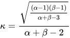
Points of inflection occur,[1][8][9][20] depending on the value of the shape parameters α and β, as follows:
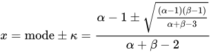
- (α > 2, β > 2) The distribution is bell-shaped (symmetric for α = β and skewed otherwise), with two inflection points, equidistant from the mode:
- (α = 2, β > 2) The distribution is unimodal, positively skewed, right-tailed, with one inflection point, located to the right of the mode:
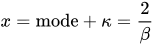
- (α > 2, β = 2) The distribution is unimodal, negatively skewed, left-tailed, with one inflection point, located to the left of the mode:
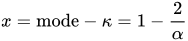
- (1 < α < 2, β > 2, α + β > 2) The distribution is unimodal, positively skewed, right-tailed, with one inflection point, located to the right of the mode:
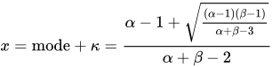
- (0 < α < 1, 1 < β < 2) The distribution has a mode at the left end x = 0 and it is positively skewed, right-tailed. There is one inflection point, located to the right of the mode:
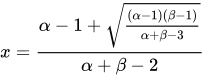
- (α > 2, 1 < β < 2) The distribution is unimodal negatively skewed, left-tailed, with one inflection point, located to the left of the mode:

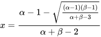
- (1 < α < 2, 0 < β < 1) The distribution has a mode at the right end x = 1 and it is negatively skewed, left-tailed. There is one inflection point, located to the left of the mode:
There are no inflection points in the remaining (symmetric and skewed) regions: U-shaped: (α, β < 1) upside-down-U-shaped: (1 < α < 2, 1 < β < 2), reverse-J-shaped (α < 1, β > 2) or J-shaped: (α > 2, β < 1)
The accompanying plots show the inflection point locations (shown vertically, ranging from 0 to 1) versus α and β (the horizontal axes ranging from 0 to 5). There are large cuts at surfaces intersecting the lines α = 1, β = 1, α = 2, and β = 2 because at these values the beta distribution change from 2 modes, to 1 mode to no mode.
Shapes


The beta density function can take a wide variety of different shapes depending on the values of the two parameters α and β. The ability of the beta distribution to take this great diversity of shapes (using only two parameters) is partly responsible for finding wide application for modeling actual measurements:
Symmetric (α = β)
- the density function is symmetric about 1/2 (blue & teal plots).
- median = mean = 1/2.
- skewness = 0.
- variance = 1/(4(2α + 1))
- α = β < 1
- U-shaped (blue plot).
- bimodal: left mode = 0, right mode =1, anti-mode = 1/2
- 1/12 < var(X) < 1/4[1]
- −2 < excess kurtosis(X) < −6/5
- α = β = 1/2 is the arcsine distribution
- var(X) = 1/8
- excess kurtosis(X) = −3/2
- CF = Rinc (t) [34]
- α = β → 0 is a 2-point Bernoulli distribution with equal probability 1/2 at each Dirac delta function end x = 0 and x = 1 and zero probability everywhere else. A coin toss: one face of the coin being x = 0 and the other face being x = 1.
- a lower value than this is impossible for any distribution to reach.
- The differential entropy approaches a minimum value of −∞
- α = β = 1
- the uniform [0, 1] distribution
- no mode
- var(X) = 1/12
- excess kurtosis(X) = −6/5
- The (negative anywhere else) differential entropy reaches its maximum value of zero
- CF = Sinc (t)
- α = β > 1
- symmetric unimodal
- mode = 1/2.
- 0 < var(X) < 1/12[1]
- −6/5 < excess kurtosis(X) < 0
- α = β = 3/2 is a semi-elliptic [0, 1] distribution, see: Wigner semicircle distribution[35]
- var(X) = 1/16.
- excess kurtosis(X) = −1
- CF = 2 Jinc (t)
- α = β = 2 is the parabolic [0, 1] distribution
- var(X) = 1/20
- excess kurtosis(X) = −6/7
- CF = 3 Tinc (t) [36]
- α = β > 2 is bell-shaped, with inflection points located to either side of the mode
- 0 < var(X) < 1/20
- −6/7 < excess kurtosis(X) < 0
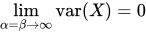
- α = β → ∞ is a 1-point Degenerate distribution with a Dirac delta function spike at the midpoint x = 1/2 with probability 1, and zero probability everywhere else. There is 100% probability (absolute certainty) concentrated at the single point x = 1/2.
- The differential entropy approaches a minimum value of −∞


Skewed (α ≠ β)
The density function is skewed. An interchange of parameter values yields the mirror image (the reverse) of the initial curve, some more specific cases:
- α < 1, β < 1
- U-shaped
- Positive skew for α < β, negative skew for α > β.
- bimodal: left mode = 0, right mode = 1, anti-mode =
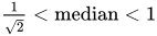
- 0 < median < 1.
- 0 < var(X) < 1/4
- α > 1, β > 1
- unimodal (magenta & cyan plots),
- Positive skew for α < β, negative skew for α > β.
- 0 < median < 1
- 0 < var(X) < 1/12
- α < 1, β ≥ 1
- reverse J-shaped with a right tail,
- positively skewed,
- strictly decreasing, convex
- mode = 0
- 0 < median < 1/2.
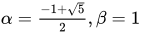
- (maximum variance occurs for , or α = Φ the golden ratio conjugate)
- α ≥ 1, β < 1
- J-shaped with a left tail,
- negatively skewed,
- strictly increasing, convex
- mode = 1
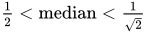
- 1/2 < median < 1
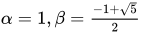
- (maximum variance occurs for , or β = Φ the golden ratio conjugate)
- α = 1, β > 1
- positively skewed,
- strictly decreasing (red plot),
- a reversed (mirror-image) power function distribution
- mean = 1 / (β + 1)
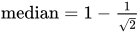
- median = 1 - 1/21/β
- mode = 0
- α = 1, 1 < β < 2
- concave
- 1/18 < var(X) < 1/12.
- α = 1, β = 2
- a straight line with slope −2, the right-triangular distribution with right angle at the left end, at x = 0
- var(X) = 1/18
- α = 1, β > 2
- reverse J-shaped with a right tail,
- convex
- 0 < var(X) < 1/18
- α > 1, β = 1
- negatively skewed,
- strictly increasing (green plot),
- the power function distribution[9]
- mean = α / (α + 1)
- median = 1/21/α
- mode = 1
- 2 > α > 1, β = 1
- concave
- 1/18 < var(X) < 1/12
- α = 2, β = 1
- a straight line with slope +2, the right-triangular distribution with right angle at the right end, at x = 1
- var(X) = 1/18
- α > 2, β = 1
- J-shaped with a left tail, convex
- 0 < var(X) < 1/18





Related distributions
Transformations
- If X ~ Beta(α, β) then 1 − X ~ Beta(β, α) mirror-image symmetry
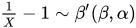
- If X ~ Beta(α, β) then . The beta prime distribution, also called "beta distribution of the second kind".
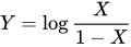
- If , then has a generalized logistic distribution, also called logistic-beta, with density , where is the logistic sigmoid.
- If X ~ Beta(α, β) then .
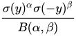
- If and then has density for and for , where is the Hypergeometric function.[37]
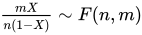
- If X ~ Beta(n/2, m/2) then (assuming n > 0 and m > 0), the Fisher–Snedecor F distribution.
- If then min + X(max − min) ~ PERT(min, max, m, λ) where PERT denotes a PERT distribution used in PERT analysis, and m=most likely value.[38] Traditionally[39]λ = 4 in PERT analysis.
- If X ~ Beta(1, β) then X ~ Kumaraswamy distribution with parameters (1, β)
- If X ~ Beta(α, 1) then X ~ Kumaraswamy distribution with parameters (α, 1)
- If X ~ Beta(α, 1) then −ln(X) ~ Exponential(α)






Special and limiting cases
- Beta(1, 1) ~ U(0, 1) with density 1 on that interval.
- Beta(n, 1) ~ Maximum of n independent rvs. with U(0, 1), sometimes called a a standard power function distribution with density n xn–1 on that interval.
- Beta(1, n) ~ Minimum of n independent rvs. with U(0, 1) with density n(1 − x)n−1 on that interval.
- If X ~ Beta(3/2, 3/2) and r > 0 then 2rX − r ~ Wigner semicircle distribution.
- Beta(1/2, 1/2) is equivalent to the arcsine distribution. This distribution is also Jeffreys prior probability for the Bernoulli and binomial distributions.
- the exponential distribution.
- the gamma distribution.
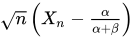
- For large , the normal distribution. More precisely, if then converges in distribution to a normal distribution with mean 0 and variance as n increases.






Derived from other distributions
- The kth order statistic of a sample of size n from the uniform distribution is a beta random variable, U(k) ~ Beta(k, n+1−k).[40]
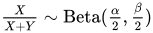
- Gamma distribution: If X ~ Gamma(α, θ) and Y ~ Gamma(β, θ) are independent, then .
- Chi-squared distribution: If and are independent, then .
- The power transformation for the uniform distribution: If X ~ U(0, 1) and α > 0 then X1/α ~ Beta(α, 1).
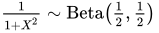
- Cauchy distribution: If X ~ Cauchy(0, 1) then



Combination with other distributions
- X ~ Beta(α, β) and Y ~ F(2β,2α) then for all x > 0.

Compounding with other distributions
- If p ~ Beta(α, β) and X ~ Bin(k, p) then X ~ beta-binomial distribution
- If p ~ Beta(α, β) and X ~ NB(r, p) then X ~ beta negative binomial distribution
Generalisations
- The multivariate generalization with sum-to-1 constraint is called a Dirichlet distribution. Univariate marginals of the Dirichlet distribution have a beta distribution. The beta distribution is conjugate to the binomial and Bernoulli distributions in exactly the same way as the Dirichlet distribution is conjugate to the multinomial distribution and categorical distribution.
- The multivariate Logistic-beta distribution[41] along with coordinate-wise logistic transformation can be considered as a multivariate generalization of beta distribution without sum-to-1 constraint. It is supported on the unit hypercube with common Beta(α, β) univariate marginals.
- The Pearson type I distribution is identical to the beta distribution (except for arbitrary shifting and re-scaling that can also be accomplished with the four parameter parametrization of the beta distribution).
- The beta distribution is the special case of the noncentral beta distribution where : .
- The generalized beta distribution is a five-parameter distribution family which has the beta distribution as a special case.
- The matrix variate beta distribution is a distribution for positive-definite matrices.


Statistical inference
Parameter estimation
Method of moments
Two unknown parameters
Two unknown parameters ( of a beta distribution supported in the [0,1] interval) can be estimated, using the method of moments, with the first two moments (sample mean and sample variance) as follows. Let:

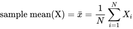
be the sample mean estimate and

be the sample variance estimate. The method-of-moments estimates of the parameters are


When the distribution is required over a known interval other than [0, 1] with random variable X, say [a, c] with random variable Y, then replace with and with in the above couple of equations for the shape parameters (see the "Four unknown parameters" section below),[42] where:


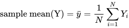

Four unknown parameters
All four parameters ( of a beta distribution supported in the [a, c] interval, see section "Alternative parametrizations, Four parameters") can be estimated, using the method of moments developed by Karl Pearson, by equating sample and population values of the first four central moments (mean, variance, skewness and excess kurtosis).[1][43][44] The excess kurtosis was expressed in terms of the square of the skewness, and the sample size ν = α + β, (see previous section "Kurtosis") as follows:


One can use this equation to solve for the sample size ν= α + β in terms of the square of the skewness and the excess kurtosis as follows:[43]


This is the ratio (multiplied by a factor of 3) between the previously derived limit boundaries for the beta distribution in a space (as originally done by Karl Pearson[21]) defined with coordinates of the square of the skewness in one axis and the excess kurtosis in the other axis (see § Kurtosis bounded by the square of the skewness):
The case of zero skewness, can be immediately solved because for zero skewness, α = β and hence ν = 2α = 2β, therefore α = β = ν/2


(Excess kurtosis is negative for the beta distribution with zero skewness, ranging from -2 to 0, so that -and therefore the sample shape parameters- is positive, ranging from zero when the shape parameters approach zero and the excess kurtosis approaches -2, to infinity when the shape parameters approach infinity and the excess kurtosis approaches zero).

For non-zero sample skewness one needs to solve a system of two coupled equations. Since the skewness and the excess kurtosis are independent of the parameters , the parameters can be uniquely determined from the sample skewness and the sample excess kurtosis, by solving the coupled equations with two known variables (sample skewness and sample excess kurtosis) and two unknowns (the shape parameters):


resulting in the following solution:[43]
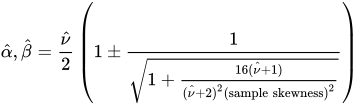

Where one should take the solutions as follows: for (negative) sample skewness < 0, and for (positive) sample skewness > 0.


The accompanying plot shows these two solutions as surfaces in a space with horizontal axes of (sample excess kurtosis) and (sample squared skewness) and the shape parameters as the vertical axis. The surfaces are constrained by the condition that the sample excess kurtosis must be bounded by the sample squared skewness as stipulated in the above equation. The two surfaces meet at the right edge defined by zero skewness. Along this right edge, both parameters are equal and the distribution is symmetric U-shaped for α = β < 1, uniform for α = β = 1, upside-down-U-shaped for 1 < α = β < 2 and bell-shaped for α = β > 2. The surfaces also meet at the front (lower) edge defined by "the impossible boundary" line (excess kurtosis + 2 - skewness2 = 0). Along this front (lower) boundary both shape parameters approach zero, and the probability density is concentrated more at one end than the other end (with practically nothing in between), with probabilities at the left end x = 0 and at the right end x = 1. The two surfaces become further apart towards the rear edge. At this rear edge the surface parameters are quite different from each other. As remarked, for example, by Bowman and Shenton,[45] sampling in the neighborhood of the line (sample excess kurtosis - (3/2)(sample skewness)2 = 0) (the just-J-shaped portion of the rear edge where blue meets beige), "is dangerously near to chaos", because at that line the denominator of the expression above for the estimate ν = α + β becomes zero and hence ν approaches infinity as that line is approached. Bowman and Shenton [45] write that "the higher moment parameters (kurtosis and skewness) are extremely fragile (near that line). However, the mean and standard deviation are fairly reliable." Therefore, the problem is for the case of four parameter estimation for very skewed distributions such that the excess kurtosis approaches (3/2) times the square of the skewness. This boundary line is produced by extremely skewed distributions with very large values of one of the parameters and very small values of the other parameter. See § Kurtosis bounded by the square of the skewness for a numerical example and further comments about this rear edge boundary line (sample excess kurtosis - (3/2)(sample skewness)2 = 0). As remarked by Karl Pearson himself [46] this issue may not be of much practical importance as this trouble arises only for very skewed J-shaped (or mirror-image J-shaped) distributions with very different values of shape parameters that are unlikely to occur much in practice). The usual skewed-bell-shape distributions that occur in practice do not have this parameter estimation problem.
The remaining two parameters can be determined using the sample mean and the sample variance using a variety of equations.[1][43] One alternative is to calculate the support interval range based on the sample variance and the sample kurtosis. For this purpose one can solve, in terms of the range , the equation expressing the excess kurtosis in terms of the sample variance, and the sample size ν (see § Kurtosis and § Alternative parametrizations, four parameters):


to obtain:

Another alternative is to calculate the support interval range based on the sample variance and the sample skewness.[43] For this purpose one can solve, in terms of the range , the equation expressing the squared skewness in terms of the sample variance, and the sample size ν (see section titled "Skewness" and "Alternative parametrizations, four parameters"):

to obtain:[43]

The remaining parameter can be determined from the sample mean and the previously obtained parameters: :


and finally, .

In the above formulas one may take, for example, as estimates of the sample moments:
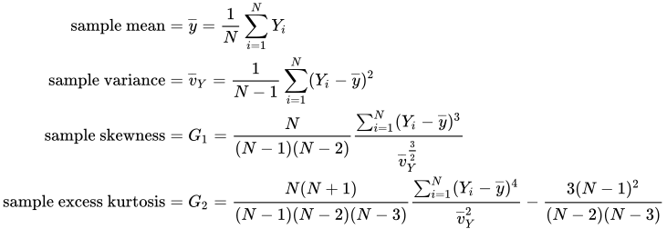
The estimators G1 for sample skewness and G2 for sample kurtosis are used by DAP/SAS, PSPP/SPSS, and Excel. However, they are not used by BMDP and (according to [47]) they were not used by MINITAB in 1998. Actually, Joanes and Gill in their 1998 study[47] concluded that the skewness and kurtosis estimators used in BMDP and in MINITAB (at that time) had smaller variance and mean-squared error in normal samples, but the skewness and kurtosis estimators used in DAP/SAS, PSPP/SPSS, namely G1 and G2, had smaller mean-squared error in samples from a very skewed distribution. It is for this reason that we have spelled out "sample skewness", etc., in the above formulas, to make it explicit that the user should choose the best estimator according to the problem at hand, as the best estimator for skewness and kurtosis depends on the amount of skewness (as shown by Joanes and Gill[47]).
Maximum likelihood
Two unknown parameters


As is also the case for maximum likelihood estimates for the gamma distribution, the maximum likelihood estimates for the beta distribution do not have a general closed form solution for arbitrary values of the shape parameters. If X1, ..., XN are independent random variables each having a beta distribution, the joint log likelihood function for Niid observations is:

Finding the maximum with respect to a shape parameter involves taking the partial derivative with respect to the shape parameter and setting the expression equal to zero yielding the maximum likelihood estimator of the shape parameters:


where:
![{\displaystyle {\begin{aligned}{\frac {\partial \ln \mathrm {B} (\alpha ,\beta )}{\partial \alpha }}&=-{\frac {\partial \ln \Gamma (\alpha +\beta )}{\partial \alpha }}+{\frac {\partial \ln \Gamma (\alpha )}{\partial \alpha }}+{\frac {\partial \ln \Gamma (\beta )}{\partial \alpha }}\\[1ex]&=-\psi (\alpha +\beta )+\psi (\alpha )+0\end{aligned}}}](https://wikimedia.org/api/rest_v1/media/math/render/svg/82bf10edac73617ec99a3adbad3ff020391c4a71)
![{\displaystyle {\begin{aligned}{\frac {\partial \ln \mathrm {B} (\alpha ,\beta )}{\partial \beta }}&=-{\frac {\partial \ln \Gamma (\alpha +\beta )}{\partial \beta }}+{\frac {\partial \ln \Gamma (\alpha )}{\partial \beta }}+{\frac {\partial \ln \Gamma (\beta )}{\partial \beta }}\\[1ex]&=-\psi (\alpha +\beta )+0+\psi (\beta )\end{aligned}}}](https://wikimedia.org/api/rest_v1/media/math/render/svg/10b097547a81011b4e212824977d66b5350dc780)
since the digamma function denoted ψ(α) is defined as the logarithmic derivative of the gamma function:[18]
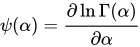
To ensure that the values with zero tangent slope are indeed a maximum (instead of a saddle-point or a minimum) one has to also satisfy the condition that the curvature is negative. This amounts to satisfying that the second partial derivative with respect to the shape parameters is negative


using the previous equations, this is equivalent to:


where the trigamma function, denoted ψ1(α), is the second of the polygamma functions, and is defined as the derivative of the digamma function:

These conditions are equivalent to stating that the variances of the logarithmically transformed variables are positive, since:
![{\displaystyle \operatorname {var} [\ln(X)]=\operatorname {E} [\ln ^{2}(X)]-(\operatorname {E} [\ln(X)])^{2}=\psi _{1}(\alpha )-\psi _{1}(\alpha +\beta )}](https://wikimedia.org/api/rest_v1/media/math/render/svg/d7737d681fea7490e27f8760c6bcc8fccb154904)
![{\displaystyle \operatorname {var} [\ln(1-X)]=\operatorname {E} [\ln ^{2}(1-X)]-(\operatorname {E} [\ln(1-X)])^{2}=\psi _{1}(\beta )-\psi _{1}(\alpha +\beta )}](https://wikimedia.org/api/rest_v1/media/math/render/svg/f84c3747955206cf2190c61bd7875a6cd739ac04)
Therefore, the condition of negative curvature at a maximum is equivalent to the statements:
![{\displaystyle \operatorname {var} [\ln(X)]>0}](https://wikimedia.org/api/rest_v1/media/math/render/svg/5fb5a5d0db057469fb9dad8df2902fe93e3f3b0d)
![{\displaystyle \operatorname {var} [\ln(1-X)]>0}](https://wikimedia.org/api/rest_v1/media/math/render/svg/c66a5aaa8362f578beb9b141b4108138b9d21e89)
Alternatively, the condition of negative curvature at a maximum is also equivalent to stating that the following logarithmic derivatives of the geometric meansGX and G(1−X) are positive, since:


While these slopes are indeed positive, the other slopes are negative:

The slopes of the mean and the median with respect to α and β display similar sign behavior.
From the condition that at a maximum, the partial derivative with respect to the shape parameter equals zero, we obtain the following system of coupled maximum likelihood estimate equations (for the average log-likelihoods) that needs to be inverted to obtain the (unknown) shape parameter estimates in terms of the (known) average of logarithms of the samples X1, ..., XN:[1]
![{\displaystyle {\begin{aligned}{\hat {\operatorname {E} }}[\ln(X)]&=\psi ({\hat {\alpha }})-\psi ({\hat {\alpha }}+{\hat {\beta }})={\frac {1}{N}}\sum _{i=1}^{N}\ln X_{i}=\ln {\hat {G}}_{X}\\{\hat {\operatorname {E} }}[\ln(1-X)]&=\psi ({\hat {\beta }})-\psi ({\hat {\alpha }}+{\hat {\beta }})={\frac {1}{N}}\sum _{i=1}^{N}\ln(1-X_{i})=\ln {\hat {G}}_{1-X}\end{aligned}}}](https://wikimedia.org/api/rest_v1/media/math/render/svg/42f099a4869ce2d200dc80c7675a237caae021e6)
where we recognize as the logarithm of the sample geometric mean and as the logarithm of the sample geometric mean based on (1 − X), the mirror-image of X. For , it follows that .


These coupled equations containing digamma functions of the shape parameter estimates must be solved by numerical methods as done, for example, by Beckman et al.[48] Gnanadesikan et al. give numerical solutions for a few cases.[49]N.L.Johnson and S.Kotz[1] suggest that for "not too small" shape parameter estimates , the logarithmic approximation to the digamma function may be used to obtain initial values for an iterative solution, since the equations resulting from this approximation can be solved exactly:

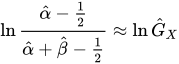

which leads to the following solution for the initial values (of the estimate shape parameters in terms of the sample geometric means) for an iterative solution:


Alternatively, the estimates provided by the method of moments can instead be used as initial values for an iterative solution of the maximum likelihood coupled equations in terms of the digamma functions.
When the distribution is required over a known interval other than [0, 1] with random variable X, say [a, c] with random variable Y, then replace ln(Xi) in the first equation with

and replace ln(1−Xi) in the second equation with

(see "Alternative parametrizations, four parameters" section below).
If one of the shape parameters is known, the problem is considerably simplified. The following logit transformation can be used to solve for the unknown shape parameter (for skewed cases such that , otherwise, if symmetric, both -equal- parameters are known when one is known):

![{\displaystyle {\hat {\operatorname {E} }}\left[\ln {\frac {X}{1-X}}\right]=\psi ({\hat {\alpha }})-\psi ({\hat {\beta }})={\frac {1}{N}}\sum _{i=1}^{N}\ln {\frac {X_{i}}{1-X_{i}}}=\ln {\hat {G}}_{X}-\ln {\hat {G}}_{1-X}}](https://wikimedia.org/api/rest_v1/media/math/render/svg/ca41c85f9e8cd1b427e96fd209fea0522c951d65)
This logit transformation is the logarithm of the transformation that divides the variable X by its mirror-image (X/(1 - X) resulting in the "inverted beta distribution" or beta prime distribution (also known as beta distribution of the second kind or Pearson's Type VI) with support [0, +∞). As previously discussed in the section "Moments of logarithmically transformed random variables," the logit transformation , studied by Johnson,[25] extends the finite support [0, 1] based on the original variable X to infinite support in both directions of the real line (−∞, +∞).

If, for example, is known, the unknown parameter can be obtained in terms of the inverse[50] digamma function of the right hand side of this equation:


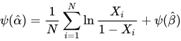

In particular, if one of the shape parameters has a value of unity, for example for (the power function distribution with bounded support [0,1]), using the identity ψ(x + 1) = ψ(x) + 1/x in the equation , the maximum likelihood estimator for the unknown parameter is,[1] exactly:


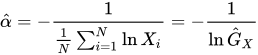
The beta has support [0, 1], therefore , and hence , and therefore

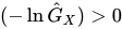

In conclusion, the maximum likelihood estimates of the shape parameters of a beta distribution are (in general) a complicated function of the sample geometric mean, and of the sample geometric mean based on (1−X)), the mirror-image of X. One may ask, if the variance (in addition to the mean) is necessary to estimate two shape parameters with the method of moments, why is the (logarithmic or geometric) variance not necessary to estimate two shape parameters with the maximum likelihood method, for which only the geometric means suffice? The answer is because the mean does not provide as much information as the geometric mean. For a beta distribution with equal shape parameters α = β, the mean is exactly 1/2, regardless of the value of the shape parameters, and therefore regardless of the value of the statistical dispersion (the variance). On the other hand, the geometric mean of a beta distribution with equal shape parameters α = β, depends on the value of the shape parameters, and therefore it contains more information. Also, the geometric mean of a beta distribution does not satisfy the symmetry conditions satisfied by the mean, therefore, by employing both the geometric mean based on X and geometric mean based on (1 − X), the maximum likelihood method is able to provide best estimates for both parameters α = β, without need of employing the variance.
One can express the joint log likelihood per Niid observations in terms of the sufficient statistics (the sample geometric means) as follows:

We can plot the joint log likelihood per N observations for fixed values of the sample geometric means to see the behavior of the likelihood function as a function of the shape parameters α and β. In such a plot, the shape parameter estimators correspond to the maxima of the likelihood function. See the accompanying graph that shows that all the likelihood functions intersect at α = β = 1, which corresponds to the values of the shape parameters that give the maximum entropy (the maximum entropy occurs for shape parameters equal to unity: the uniform distribution). It is evident from the plot that the likelihood function gives sharp peaks for values of the shape parameter estimators close to zero, but that for values of the shape parameters estimators greater than one, the likelihood function becomes quite flat, with less defined peaks. Obviously, the maximum likelihood parameter estimation method for the beta distribution becomes less acceptable for larger values of the shape parameter estimators, as the uncertainty in the peak definition increases with the value of the shape parameter estimators. One can arrive at the same conclusion by noticing that the expression for the curvature of the likelihood function is in terms of the geometric variances
![{\displaystyle {\frac {\partial ^{2}\ln {\mathcal {L}}(\alpha ,\beta \mid X)}{\partial \alpha ^{2}}}=-\operatorname {var} [\ln X]}](https://wikimedia.org/api/rest_v1/media/math/render/svg/517a09a3b13d22689a3e1e400cbcab3af08e130c)
![{\displaystyle {\frac {\partial ^{2}\ln {\mathcal {L}}(\alpha ,\beta \mid X)}{\partial \beta ^{2}}}=-\operatorname {var} [\ln(1-X)]}](https://wikimedia.org/api/rest_v1/media/math/render/svg/1715f50fc408ceba307005a3f9e404520edd5a20)
These variances (and therefore the curvatures) are much larger for small values of the shape parameter α and β. However, for shape parameter values α, β > 1, the variances (and therefore the curvatures) flatten out. Equivalently, this result follows from the Cramér–Rao bound, since the Fisher information matrix components for the beta distribution are these logarithmic variances. The Cramér–Rao bound states that the variance of any unbiased estimator of α is bounded by the reciprocal of the Fisher information:
![{\displaystyle \mathrm {var} ({\hat {\alpha }})\geq {\frac {1}{\operatorname {var} [\ln X]}}\geq {\frac {1}{\psi _{1}({\hat {\alpha }})-\psi _{1}({\hat {\alpha }}+{\hat {\beta }})}}}](https://wikimedia.org/api/rest_v1/media/math/render/svg/744f1e8421337ed7a2e6cae00fccec1eaf68e3dc)
![{\displaystyle \mathrm {var} ({\hat {\beta }})\geq {\frac {1}{\operatorname {var} [\ln(1-X)]}}\geq {\frac {1}{\psi _{1}({\hat {\beta }})-\psi _{1}({\hat {\alpha }}+{\hat {\beta }})}}}](https://wikimedia.org/api/rest_v1/media/math/render/svg/f01dc5c3eb614cfa71a500fd34f3fa430c183c76)
so the variance of the estimators increases with increasing α and β, as the logarithmic variances decrease.
Also one can express the joint log likelihood per Niid observations in terms of the digamma function expressions for the logarithms of the sample geometric means as follows:

this expression is identical to the negative of the cross-entropy (see section on "Quantities of information (entropy)"). Therefore, finding the maximum of the joint log likelihood of the shape parameters, per Niid observations, is identical to finding the minimum of the cross-entropy for the beta distribution, as a function of the shape parameters.

with the cross-entropy defined as follows:

Four unknown parameters
The procedure is similar to the one followed in the two unknown parameter case. If Y1, ..., YN are independent random variables each having a beta distribution with four parameters, the joint log likelihood function for Niid observations is:

Finding the maximum with respect to a shape parameter involves taking the partial derivative with respect to the shape parameter and setting the expression equal to zero yielding the maximum likelihood estimator of the shape parameters:




these equations can be re-arranged as the following system of four coupled equations (the first two equations are geometric means and the second two equations are the harmonic means) in terms of the maximum likelihood estimates for the four parameters :


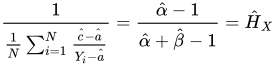
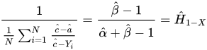
with sample geometric means:
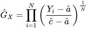
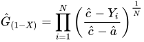
The parameters are embedded inside the geometric mean expressions in a nonlinear way (to the power 1/N). This precludes, in general, a closed form solution, even for an initial value approximation for iteration purposes. One alternative is to use as initial values for iteration the values obtained from the method of moments solution for the four parameter case. Furthermore, the expressions for the harmonic means are well-defined only for , which precludes a maximum likelihood solution for shape parameters less than unity in the four-parameter case. Fisher's information matrix for the four parameter case is positive-definite only for α, β > 2 (for further discussion, see section on Fisher information matrix, four parameter case), for bell-shaped (symmetric or unsymmetric) beta distributions, with inflection points located to either side of the mode. The following Fisher information components (that represent the expectations of the curvature of the log likelihood function) have singularities at the following values:

![{\displaystyle \alpha =2:\quad \operatorname {E} \left[-{\frac {1}{N}}{\frac {\partial ^{2}\ln {\mathcal {L}}(\alpha ,\beta ,a,c\mid Y)}{\partial a^{2}}}\right]={\mathcal {I}}_{a,a}}](https://wikimedia.org/api/rest_v1/media/math/render/svg/53538160a2404a5d7b74ae2033fbbb2dbc1045eb)
![{\displaystyle \beta =2:\quad \operatorname {E} \left[-{\frac {1}{N}}{\frac {\partial ^{2}\ln {\mathcal {L}}(\alpha ,\beta ,a,c\mid Y)}{\partial c^{2}}}\right]={\mathcal {I}}_{c,c}}](https://wikimedia.org/api/rest_v1/media/math/render/svg/ee2c6ecfcafe60e54799ab4a16451cf478d65f7d)
![{\displaystyle \alpha =2:\quad \operatorname {E} \left[-{\frac {1}{N}}{\frac {\partial ^{2}\ln {\mathcal {L}}(\alpha ,\beta ,a,c\mid Y)}{\partial \alpha \partial a}}\right]={\mathcal {I}}_{\alpha ,a}}](https://wikimedia.org/api/rest_v1/media/math/render/svg/8b8af544d7c5e0cc278aa725daba7f3de2f70d31)
![{\displaystyle \beta =1:\quad \operatorname {E} \left[-{\frac {1}{N}}{\frac {\partial ^{2}\ln {\mathcal {L}}(\alpha ,\beta ,a,c\mid Y)}{\partial \beta \partial c}}\right]={\mathcal {I}}_{\beta ,c}}](https://wikimedia.org/api/rest_v1/media/math/render/svg/2f87b32b39997964dcbc95bc64c1364e6832db1d)
(for further discussion see section on Fisher information matrix). Thus, it is not possible to strictly carry on the maximum likelihood estimation for some well known distributions belonging to the four-parameter beta distribution family, like the uniform distribution (Beta(1, 1, a, c)), and the arcsine distribution (Beta(1/2, 1/2, a, c)). N.L.Johnson and S.Kotz[1] ignore the equations for the harmonic means and instead suggest "If a and c are unknown, and maximum likelihood estimators of a, c, α and β are required, the above procedure (for the two unknown parameter case, with X transformed as X = (Y − a)/(c − a)) can be repeated using a succession of trial values of a and c, until the pair (a, c) for which maximum likelihood (given a and c) is as great as possible, is attained" (where, for the purpose of clarity, their notation for the parameters has been translated into the present notation).
Fisher information matrix
Let a random variable X have a probability density f(x;α). The partial derivative with respect to the (unknown, and to be estimated) parameter α of the log likelihood function is called the score. The second moment of the score is called the Fisher information:
![{\displaystyle {\mathcal {I}}(\alpha )=\operatorname {E} \left[\left({\frac {\partial }{\partial \alpha }}\ln {\mathcal {L}}(\alpha \mid X)\right)^{2}\right],}](https://wikimedia.org/api/rest_v1/media/math/render/svg/daec13972d17a073bcd447abfde55a6b0e168720)
The expectation of the score is zero, therefore the Fisher information is also the second moment centered on the mean of the score: the variance of the score.
If the log likelihood function is twice differentiable with respect to the parameter α, and under certain regularity conditions,[51] then the Fisher information may also be written as follows (which is often a more convenient form for calculation purposes):
![{\displaystyle {\mathcal {I}}(\alpha )=-\operatorname {E} \left[{\frac {\partial ^{2}}{\partial \alpha ^{2}}}\ln {\mathcal {L}}(\alpha \mid X)\right].}](https://wikimedia.org/api/rest_v1/media/math/render/svg/3fdd5f6730d5ffb0a5f833c89ba784362322cbc8)
Thus, the Fisher information is the negative of the expectation of the second derivative with respect to the parameter α of the log likelihood function. Therefore, Fisher information is a measure of the curvature of the log likelihood function of α. A low curvature (and therefore high radius of curvature), flatter log likelihood function curve has low Fisher information; while a log likelihood function curve with large curvature (and therefore low radius of curvature) has high Fisher information. When the Fisher information matrix is computed at the evaluates of the parameters ("the observed Fisher information matrix") it is equivalent to the replacement of the true log likelihood surface by a Taylor's series approximation, taken as far as the quadratic terms.[52] The word information, in the context of Fisher information, refers to information about the parameters. Information such as: estimation, sufficiency and properties of variances of estimators. The Cramér–Rao bound states that the inverse of the Fisher information is a lower bound on the variance of any estimator of a parameter α:
![{\displaystyle \operatorname {var} [{\hat {\alpha }}]\geq {\frac {1}{{\mathcal {I}}(\alpha )}}.}](https://wikimedia.org/api/rest_v1/media/math/render/svg/d93d4983a2717258c52eb47d1562e849a3a66c5c)
The precision to which one can estimate the estimator of a parameter α is limited by the Fisher Information of the log likelihood function. The Fisher information is a measure of the minimum error involved in estimating a parameter of a distribution and it can be viewed as a measure of the resolving power of an experiment needed to discriminate between two alternative hypothesis of a parameter.[53]
When there are N parameters
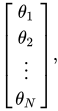
then the Fisher information takes the form of an N×Npositive semidefinitesymmetric matrix, the Fisher information matrix, with typical element:
![{\displaystyle ({\mathcal {I}}(\theta ))_{i,j}=\operatorname {E} \left[{\frac {\partial \ln {\mathcal {L}}}{\partial \theta _{i}}}\cdot {\frac {\partial \ln {\mathcal {L}}}{\partial \theta _{j}}}\right].}](https://wikimedia.org/api/rest_v1/media/math/render/svg/94187c0032daae02409e5323c356fae5fdcb73fd)
Under certain regularity conditions,[51] the Fisher Information Matrix may also be written in the following form, which is often more convenient for computation:
![{\displaystyle ({\mathcal {I}}(\theta ))_{i,j}=-\operatorname {E} \left[{\frac {\partial ^{2}\ln {\mathcal {L}}}{\partial \theta _{i}\,\partial \theta _{j}}}\right]\,.}](https://wikimedia.org/api/rest_v1/media/math/render/svg/86df084593df54dd2ed7220a683b9fbc41f230d7)
With X1, ..., XNiid random variables, an N-dimensional "box" can be constructed with sides X1, ..., XN. Costa and Cover[54] show that the (Shannon) differential entropy h(X) is related to the volume of the typical set (having the sample entropy close to the true entropy), while the Fisher information is related to the surface of this typical set.
Two parameters
For X1, ..., XN independent random variables each having a beta distribution parametrized with shape parameters α and β, the joint log likelihood function for Niid observations is:

therefore the joint log likelihood function per Niid observations is

For the two parameter case, the Fisher information has 4 components: 2 diagonal and 2 off-diagonal. Since the Fisher information matrix is symmetric, one of these off diagonal components is independent. Therefore, the Fisher information matrix has 3 independent components (2 diagonal and 1 off diagonal).
Aryal and Nadarajah[55] calculated Fisher's information matrix for the four-parameter case, from which the two parameter case can be obtained as follows:
![{\displaystyle -{\frac {\partial ^{2}\ln {\mathcal {L}}(\alpha ,\beta \mid X)}{N\partial \alpha ^{2}}}=\operatorname {var} [\ln(X)]=\psi _{1}(\alpha )-\psi _{1}(\alpha +\beta )={\mathcal {I}}_{\alpha ,\alpha }=\operatorname {E} \left[-{\frac {\partial ^{2}\ln {\mathcal {L}}(\alpha ,\beta \mid X)}{N\partial \alpha ^{2}}}\right]=\ln \operatorname {var} _{GX}}](https://wikimedia.org/api/rest_v1/media/math/render/svg/c90003d5bd2f6d2bcfe2c788585689726b4b7e36)
![{\displaystyle -{\frac {\partial ^{2}\ln {\mathcal {L}}(\alpha ,\beta \mid X)}{N\,\partial \beta ^{2}}}=\operatorname {var} [\ln(1-X)]=\psi _{1}(\beta )-\psi _{1}(\alpha +\beta )={\mathcal {I}}_{\beta ,\beta }=\operatorname {E} \left[-{\frac {\partial ^{2}\ln {\mathcal {L}}(\alpha ,\beta \mid X)}{N\partial \beta ^{2}}}\right]=\ln \operatorname {var} _{G(1-X)}}](https://wikimedia.org/api/rest_v1/media/math/render/svg/b59bcc31f14f1f4b3b07bd92a66426bb6ac126b1)
![{\displaystyle -{\frac {\partial ^{2}\ln {\mathcal {L}}(\alpha ,\beta \mid X)}{N\,\partial \alpha \,\partial \beta }}=\operatorname {cov} [\ln X,\ln(1-X)]=-\psi _{1}(\alpha +\beta )={\mathcal {I}}_{\alpha ,\beta }=\operatorname {E} \left[-{\frac {\partial ^{2}\ln {\mathcal {L}}(\alpha ,\beta \mid X)}{N\,\partial \alpha \,\partial \beta }}\right]=\ln \operatorname {cov} _{G{X,(1-X)}}}](https://wikimedia.org/api/rest_v1/media/math/render/svg/a6c3268da3b23c062ce981ab02d4c454a0267365)
Since the Fisher information matrix is symmetric

The Fisher information components are equal to the log geometric variances and log geometric covariance. Therefore, they can be expressed as trigamma functions, denoted ψ1(α), the second of the polygamma functions, defined as the derivative of the digamma function:
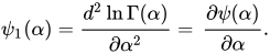
These derivatives are also derived in the § Two unknown parameters and plots of the log likelihood function are also shown in that section. § Geometric variance and covariance contains plots and further discussion of the Fisher information matrix components: the log geometric variances and log geometric covariance as a function of the shape parameters α and β. § Moments of logarithmically transformed random variables contains formulas for moments of logarithmically transformed random variables. Images for the Fisher information components and are shown in § Geometric variance.


The determinant of Fisher's information matrix is of interest (for example for the calculation of Jeffreys prior probability). From the expressions for the individual components of the Fisher information matrix, it follows that the determinant of Fisher's (symmetric) information matrix for the beta distribution is:
![{\displaystyle {\begin{aligned}\det({\mathcal {I}}(\alpha ,\beta ))&={\mathcal {I}}_{\alpha ,\alpha }{\mathcal {I}}_{\beta ,\beta }-{\mathcal {I}}_{\alpha ,\beta }{\mathcal {I}}_{\alpha ,\beta }\\[4pt]&=(\psi _{1}(\alpha )-\psi _{1}(\alpha +\beta ))(\psi _{1}(\beta )-\psi _{1}(\alpha +\beta ))-(-\psi _{1}(\alpha +\beta ))(-\psi _{1}(\alpha +\beta ))\\[4pt]&=\psi _{1}(\alpha )\psi _{1}(\beta )-(\psi _{1}(\alpha )+\psi _{1}(\beta ))\psi _{1}(\alpha +\beta )\\[4pt]\lim _{\alpha \to 0}\det({\mathcal {I}}(\alpha ,\beta ))&=\lim _{\beta \to 0}\det({\mathcal {I}}(\alpha ,\beta ))=\infty \\[4pt]\lim _{\alpha \to \infty }\det({\mathcal {I}}(\alpha ,\beta ))&=\lim _{\beta \to \infty }\det({\mathcal {I}}(\alpha ,\beta ))=0\end{aligned}}}](https://wikimedia.org/api/rest_v1/media/math/render/svg/b2c5ccf59b05ea730fc108360c07e9ac9634e829)
From Sylvester's criterion (checking whether the diagonal elements are all positive), it follows that the Fisher information matrix for the two parameter case is positive-definite (under the standard condition that the shape parameters are positive α > 0 and β > 0).
Four parameters


If Y1, ..., YN are independent random variables each having a beta distribution with four parameters: the exponents α and β, and also a (the minimum of the distribution range), and c (the maximum of the distribution range) (section titled "Alternative parametrizations", "Four parameters"), with probability density function:

the joint log likelihood function per Niid observations is:

For the four parameter case, the Fisher information has 4*4=16 components. It has 12 off-diagonal components = (4×4 total − 4 diagonal). Since the Fisher information matrix is symmetric, half of these components (12/2=6) are independent. Therefore, the Fisher information matrix has 6 independent off-diagonal + 4 diagonal = 10 independent components. Aryal and Nadarajah[55] calculated Fisher's information matrix for the four parameter case as follows:
![{\displaystyle -{\frac {1}{N}}{\frac {\partial ^{2}\ln {\mathcal {L}}(\alpha ,\beta ,a,c\mid Y)}{\partial \alpha ^{2}}}=\operatorname {var} [\ln(X)]=\psi _{1}(\alpha )-\psi _{1}(\alpha +\beta )={\mathcal {I}}_{\alpha ,\alpha }=\operatorname {E} \left[-{\frac {1}{N}}{\frac {\partial ^{2}\ln {\mathcal {L}}(\alpha ,\beta ,a,c\mid Y)}{\partial \alpha ^{2}}}\right]=\ln(\operatorname {var_{GX}} )}](https://wikimedia.org/api/rest_v1/media/math/render/svg/31be86f2c53663c6d3975bc2676806ba3e538423)
![{\displaystyle -{\frac {1}{N}}{\frac {\partial ^{2}\ln {\mathcal {L}}(\alpha ,\beta ,a,c\mid Y)}{\partial \beta ^{2}}}=\operatorname {var} [\ln(1-X)]=\psi _{1}(\beta )-\psi _{1}(\alpha +\beta )={\mathcal {I}}_{\beta ,\beta }=\operatorname {E} \left[-{\frac {1}{N}}{\frac {\partial ^{2}\ln {\mathcal {L}}(\alpha ,\beta ,a,c\mid Y)}{\partial \beta ^{2}}}\right]=\ln(\operatorname {var_{G(1-X)}} )}](https://wikimedia.org/api/rest_v1/media/math/render/svg/25ab885119f25fae0b9919326db96395d13e3bc3)
![{\displaystyle -{\frac {1}{N}}{\frac {\partial ^{2}\ln {\mathcal {L}}(\alpha ,\beta ,a,c\mid Y)}{\partial \alpha \,\partial \beta }}=\operatorname {cov} [\ln X,(1-X)]=-\psi _{1}(\alpha +\beta )={\mathcal {I}}_{\alpha ,\beta }=\operatorname {E} \left[-{\frac {1}{N}}{\frac {\partial ^{2}\ln {\mathcal {L}}(\alpha ,\beta ,a,c\mid Y)}{\partial \alpha \,\partial \beta }}\right]=\ln(\operatorname {cov} _{G{X,(1-X)}})}](https://wikimedia.org/api/rest_v1/media/math/render/svg/02a56af746fb9315340cf382951fe0c3f3640678)
In the above expressions, the use of X instead of Y in the expressions var[ln(X)] = ln(varGX) is not an error. The expressions in terms of the log geometric variances and log geometric covariance occur as functions of the two parameter X ~ Beta(α, β) parametrization because when taking the partial derivatives with respect to the exponents (α, β) in the four parameter case, one obtains the identical expressions as for the two parameter case: these terms of the four parameter Fisher information matrix are independent of the minimum a and maximum c of the distribution's range. The only non-zero term upon double differentiation of the log likelihood function with respect to the exponents α and β is the second derivative of the log of the beta function: ln(B(α, β)). This term is independent of the minimum a and maximum c of the distribution's range. Double differentiation of this term results in trigamma functions. The sections titled "Maximum likelihood", "Two unknown parameters" and "Four unknown parameters" also show this fact.
The Fisher information for Ni.i.d. samples is N times the individual Fisher information (eq. 11.279, page 394 of Cover and Thomas[28]). (Aryal and Nadarajah[55] take a single observation, N = 1, to calculate the following components of the Fisher information, which leads to the same result as considering the derivatives of the log likelihood per N observations. Moreover, below the erroneous expression for in Aryal and Nadarajah has been corrected.)

![{\displaystyle {\begin{aligned}\alpha >2:\quad \operatorname {E} \left[-{\frac {1}{N}}{\frac {\partial ^{2}\ln {\mathcal {L}}(\alpha ,\beta ,a,c\mid Y)}{\partial a^{2}}}\right]&={\mathcal {I}}_{a,a}={\frac {\beta (\alpha +\beta -1)}{(\alpha -2)(c-a)^{2}}}\\\beta >2:\quad \operatorname {E} \left[-{\frac {1}{N}}{\frac {\partial ^{2}\ln {\mathcal {L}}(\alpha ,\beta ,a,c\mid Y)}{\partial c^{2}}}\right]&={\mathcal {I}}_{c,c}={\frac {\alpha (\alpha +\beta -1)}{(\beta -2)(c-a)^{2}}}\\\operatorname {E} \left[-{\frac {1}{N}}{\frac {\partial ^{2}\ln {\mathcal {L}}(\alpha ,\beta ,a,c\mid Y)}{\partial a\,\partial c}}\right]&={\mathcal {I}}_{a,c}={\frac {(\alpha +\beta -1)}{(c-a)^{2}}}\\\alpha >1:\quad \operatorname {E} \left[-{\frac {1}{N}}{\frac {\partial ^{2}\ln {\mathcal {L}}(\alpha ,\beta ,a,c\mid Y)}{\partial \alpha \,\partial a}}\right]&={\mathcal {I}}_{\alpha ,a}={\frac {\beta }{(\alpha -1)(c-a)}}\\\operatorname {E} \left[-{\frac {1}{N}}{\frac {\partial ^{2}\ln {\mathcal {L}}(\alpha ,\beta ,a,c\mid Y)}{\partial \alpha \,\partial c}}\right]&={\mathcal {I}}_{\alpha ,c}={\frac {1}{(c-a)}}\\\operatorname {E} \left[-{\frac {1}{N}}{\frac {\partial ^{2}\ln {\mathcal {L}}(\alpha ,\beta ,a,c\mid Y)}{\partial \beta \,\partial a}}\right]&={\mathcal {I}}_{\beta ,a}=-{\frac {1}{(c-a)}}\\\beta >1:\quad \operatorname {E} \left[-{\frac {1}{N}}{\frac {\partial ^{2}\ln {\mathcal {L}}(\alpha ,\beta ,a,c\mid Y)}{\partial \beta \,\partial c}}\right]&={\mathcal {I}}_{\beta ,c}=-{\frac {\alpha }{(\beta -1)(c-a)}}\end{aligned}}}](https://wikimedia.org/api/rest_v1/media/math/render/svg/636646f51bdb1a3193b1721483878e98f4f19c3e)
The lower two diagonal entries of the Fisher information matrix, with respect to the parameter a (the minimum of the distribution's range): , and with respect to the parameter c (the maximum of the distribution's range): are only defined for exponents α > 2 and β > 2 respectively. The Fisher information matrix component for the minimum a approaches infinity for exponent α approaching 2 from above, and the Fisher information matrix component for the maximum c approaches infinity for exponent β approaching 2 from above.

The Fisher information matrix for the four parameter case does not depend on the individual values of the minimum a and the maximum c, but only on the total range (c − a). Moreover, the components of the Fisher information matrix that depend on the range (c − a), depend only through its inverse (or the square of the inverse), such that the Fisher information decreases for increasing range (c − a).
The accompanying images show the Fisher information components and . Images for the Fisher information components and are shown in § Geometric variance. All these Fisher information components look like a basin, with the "walls" of the basin being located at low values of the parameters.


The following four-parameter-beta-distribution Fisher information components can be expressed in terms of the two-parameter: X ~ Beta(α, β) expectations of the transformed ratio ((1 − X)/X) and of its mirror image (X/(1 − X)), scaled by the range (c − a), which may be helpful for interpretation:
![{\displaystyle {\mathcal {I}}_{\alpha ,a}={\frac {\operatorname {E} \left[{\frac {1-X}{X}}\right]}{c-a}}={\frac {\beta }{(\alpha -1)(c-a)}}{\text{ if }}\alpha >1}](https://wikimedia.org/api/rest_v1/media/math/render/svg/e670565bb8d06bace69cf892864520f5c83b5449)
![{\displaystyle {\mathcal {I}}_{\beta ,c}=-{\frac {\operatorname {E} \left[{\frac {X}{1-X}}\right]}{c-a}}=-{\frac {\alpha }{(\beta -1)(c-a)}}{\text{ if }}\beta >1}](https://wikimedia.org/api/rest_v1/media/math/render/svg/94f9b7788a4f19e1cbc765ab8fc85a7ad55dec4f)
These are also the expected values of the "inverted beta distribution" or beta prime distribution (also known as beta distribution of the second kind or Pearson's Type VI) [1] and its mirror image, scaled by the range (c − a).
Also, the following Fisher information components can be expressed in terms of the harmonic (1/X) variances or of variances based on the ratio transformed variables ((1-X)/X) as follows:
![{\displaystyle {\begin{aligned}\alpha >2:\quad {\mathcal {I}}_{a,a}&=\operatorname {var} \left[{\frac {1}{X}}\right]\left({\frac {\alpha -1}{c-a}}\right)^{2}=\operatorname {var} \left[{\frac {1-X}{X}}\right]\left({\frac {\alpha -1}{c-a}}\right)^{2}={\frac {\beta (\alpha +\beta -1)}{(\alpha -2)(c-a)^{2}}}\\\beta >2:\quad {\mathcal {I}}_{c,c}&=\operatorname {var} \left[{\frac {1}{1-X}}\right]\left({\frac {\beta -1}{c-a}}\right)^{2}=\operatorname {var} \left[{\frac {X}{1-X}}\right]\left({\frac {\beta -1}{c-a}}\right)^{2}={\frac {\alpha (\alpha +\beta -1)}{(\beta -2)(c-a)^{2}}}\\{\mathcal {I}}_{a,c}&=\operatorname {cov} \left[{\frac {1}{X}},{\frac {1}{1-X}}\right]{\frac {(\alpha -1)(\beta -1)}{(c-a)^{2}}}=\operatorname {cov} \left[{\frac {1-X}{X}},{\frac {X}{1-X}}\right]{\frac {(\alpha -1)(\beta -1)}{(c-a)^{2}}}={\frac {(\alpha +\beta -1)}{(c-a)^{2}}}\end{aligned}}}](https://wikimedia.org/api/rest_v1/media/math/render/svg/f1f89730020364bb58791ca0eb47d0de25c896c2)
See section "Moments of linearly transformed, product and inverted random variables" for these expectations.
The determinant of Fisher's information matrix is of interest (for example for the calculation of Jeffreys prior probability). From the expressions for the individual components, it follows that the determinant of Fisher's (symmetric) information matrix for the beta distribution with four parameters is:
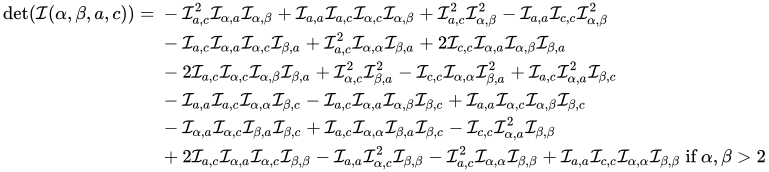
Using Sylvester's criterion (checking whether the diagonal elements are all positive), and since diagonal components and have singularities at α=2 and β=2 it follows that the Fisher information matrix for the four parameter case is positive-definite for α>2 and β>2. Since for α > 2 and β > 2 the beta distribution is (symmetric or unsymmetric) bell shaped, it follows that the Fisher information matrix is positive-definite only for bell-shaped (symmetric or unsymmetric) beta distributions, with inflection points located to either side of the mode. Thus, important well known distributions belonging to the four-parameter beta distribution family, like the parabolic distribution (Beta(2,2,a,c)) and the uniform distribution (Beta(1,1,a,c)) have Fisher information components () that blow up (approach infinity) in the four-parameter case (although their Fisher information components are all defined for the two parameter case). The four-parameter Wigner semicircle distribution (Beta(3/2,3/2,a,c)) and arcsine distribution (Beta(1/2,1/2,a,c)) have negative Fisher information determinants for the four-parameter case.

Bayesian inference


The use of Beta distributions in Bayesian inference is due to the fact that they provide a family of conjugate prior probability distributions for binomial (including Bernoulli) and geometric distributions. The domain of the beta distribution can be viewed as a probability, and in fact the beta distribution is often used to describe the distribution of a probability value p:[24]
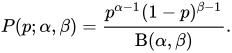
Examples of beta distributions used as prior probabilities to represent ignorance of prior parameter values in Bayesian inference are Beta(1,1), Beta(0,0) and Beta(1/2,1/2).
Rule of succession
A classic application of the beta distribution is the rule of succession, introduced in the 18th century by Pierre-Simon Laplace[56] in the course of treating the sunrise problem. It states that, given s successes in nconditionally independentBernoulli trials with probability p, that the estimate of the expected value in the next trial is . This estimate is the expected value of the posterior distribution over p, namely Beta(s+1, n−s+1), which is given by Bayes' rule if one assumes a uniform prior probability over p (i.e., Beta(1, 1)) and then observes that p generated s successes in n trials. Laplace's rule of succession has been criticized by prominent scientists. R. T. Cox described Laplace's application of the rule of succession to the sunrise problem ([57] p. 89) as "a travesty of the proper use of the principle". Keynes remarks ([58] Ch.XXX, p. 382) "indeed this is so foolish a theorem that to entertain it is discreditable". Karl Pearson[59] showed that the probability that the next (n + 1) trials will be successes, after n successes in n trials, is only 50%, which has been considered too low by scientists like Jeffreys and unacceptable as a representation of the scientific process of experimentation to test a proposed scientific law. As pointed out by Jeffreys ([60] p. 128) (crediting C. D. Broad[61] ) Laplace's rule of succession establishes a high probability of success ((n+1)/(n+2)) in the next trial, but only a moderate probability (50%) that a further sample (n+1) comparable in size will be equally successful. As pointed out by Perks,[62] "The rule of succession itself is hard to accept. It assigns a probability to the next trial which implies the assumption that the actual run observed is an average run and that we are always at the end of an average run. It would, one would think, be more reasonable to assume that we were in the middle of an average run. Clearly a higher value for both probabilities is necessary if they are to accord with reasonable belief." These problems with Laplace's rule of succession motivated Haldane, Perks, Jeffreys and others to search for other forms of prior probability (see the next § Bayesian inference). According to Jaynes,[53] the main problem with the rule of succession is that it is not valid when s=0 or s=n (see rule of succession, for an analysis of its validity).

Bayes–Laplace prior probability (Beta(1,1))
The beta distribution achieves maximum differential entropy for Beta(1,1): the uniform probability density, for which all values in the domain of the distribution have equal density. This uniform distribution Beta(1,1) was suggested ("with a great deal of doubt") by Thomas Bayes[63] as the prior probability distribution to express ignorance about the correct prior distribution. This prior distribution was adopted (apparently, from his writings, with little sign of doubt[56]) by Pierre-Simon Laplace, and hence it was also known as the "Bayes–Laplace rule" or the "Laplace rule" of "inverse probability" in publications of the first half of the 20th century. In the later part of the 19th century and early part of the 20th century, scientists realized that the assumption of uniform "equal" probability density depended on the actual functions (for example whether a linear or a logarithmic scale was most appropriate) and parametrizations used. In particular, the behavior near the ends of distributions with finite support (for example near x = 0, for a distribution with initial support at x = 0) required particular attention. Keynes ([58] Ch.XXX, p. 381) criticized the use of Bayes's uniform prior probability (Beta(1,1)) that all values between zero and one are equiprobable, as follows: "Thus experience, if it shows anything, shows that there is a very marked clustering of statistical ratios in the neighborhoods of zero and unity, of those for positive theories and for correlations between positive qualities in the neighborhood of zero, and of those for negative theories and for correlations between negative qualities in the neighborhood of unity. "
Haldane's prior probability (Beta(0,0))


The Beta(0,0) distribution was proposed by J.B.S. Haldane,[64] who suggested that the prior probability representing complete uncertainty should be proportional to p−1(1−p)−1. The function p−1(1−p)−1 can be viewed as the limit of the numerator of the beta distribution as both shape parameters approach zero: α, β → 0. The Beta function (in the denominator of the beta distribution) approaches infinity, for both parameters approaching zero, α, β → 0. Therefore, p−1(1−p)−1 divided by the Beta function approaches a 2-point Bernoulli distribution with equal probability 1/2 at each end, at 0 and 1, and nothing in between, as α, β → 0. A coin-toss: one face of the coin being at 0 and the other face being at 1. The Haldane prior probability distribution Beta(0,0) is an "improper prior" because its integration (from 0 to 1) fails to strictly converge to 1 due to the singularities at each end. However, this is not an issue for computing posterior probabilities unless the sample size is very small. Furthermore, Zellner[65] points out that on the log-odds scale, (the logit transformation ), the Haldane prior is the uniformly flat prior. The fact that a uniform prior probability on the logit transformed variable ln(p/1 − p) (with domain (−∞, ∞)) is equivalent to the Haldane prior on the domain [0, 1] was pointed out by Harold Jeffreys in the first edition (1939) of his book Theory of Probability ([60] p. 123). Jeffreys writes "Certainly if we take the Bayes–Laplace rule right up to the extremes we are led to results that do not correspond to anybody's way of thinking. The (Haldane) rule dx/(x(1 − x)) goes too far the other way. It would lead to the conclusion that if a sample is of one type with respect to some property there is a probability 1 that the whole population is of that type." The fact that "uniform" depends on the parametrization, led Jeffreys to seek a form of prior that would be invariant under different parametrizations.

Jeffreys' prior probability (Beta(1/2,1/2) for a Bernoulli or for a binomial distribution)




Harold Jeffreys[60][66] proposed to use an uninformative prior probability measure that should be invariant under reparameterization: proportional to the square root of the determinant of Fisher's information matrix. For the Bernoulli distribution, this can be shown as follows: for a coin that is "heads" with probability p ∈ [0, 1] and is "tails" with probability 1 − p, for a given (H,T) ∈ {(0,1), (1,0)} the probability is pH(1 − p)T. Since T = 1 − H, the Bernoulli distribution is pH(1 − p)1 − H. Considering p as the only parameter, it follows that the log likelihood for the Bernoulli distribution is

The Fisher information matrix has only one component (it is a scalar, because there is only one parameter: p), therefore:
![{\displaystyle {\begin{aligned}{\sqrt {{\mathcal {I}}(p)}}&={\sqrt {\operatorname {E} \!\left[\left({\frac {d}{dp}}\ln {\mathcal {L}}(p\mid H)\right)^{2}\right]}}\\[6pt]&={\sqrt {\operatorname {E} \!\left[\left({\frac {H}{p}}-{\frac {1-H}{1-p}}\right)^{2}\right]}}\\[6pt]&={\sqrt {p^{1}(1-p)^{0}\left({\frac {1}{p}}-{\frac {0}{1-p}}\right)^{2}+p^{0}(1-p)^{1}\left({\frac {0}{p}}-{\frac {1}{1-p}}\right)^{2}}}\\&={\frac {1}{\sqrt {p(1-p)}}}.\end{aligned}}}](https://wikimedia.org/api/rest_v1/media/math/render/svg/0c2541cc4a3017abaab79170bd990ca92a64bc89)
Similarly, for the Binomial distribution with nBernoulli trials, it can be shown that

Thus, for the Bernoulli, and Binomial distributions, Jeffreys prior is proportional to , which happens to be proportional to a beta distribution with domain variable x = p, and shape parameters α = β = 1/2, the arcsine distribution:


It will be shown in the next section that the normalizing constant for Jeffreys prior is immaterial to the final result because the normalizing constant cancels out in Bayes' theorem for the posterior probability. Hence Beta(1/2,1/2) is used as the Jeffreys prior for both Bernoulli and binomial distributions. As shown in the next section, when using this expression as a prior probability times the likelihood in Bayes' theorem, the posterior probability turns out to be a beta distribution. It is important to realize, however, that Jeffreys prior is proportional to for the Bernoulli and binomial distribution, but not for the beta distribution. Jeffreys prior for the beta distribution is given by the determinant of Fisher's information for the beta distribution, which, as shown in the § Fisher information matrix is a function of the trigamma function ψ1 of shape parameters α and β as follows:

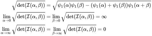
As previously discussed, Jeffreys prior for the Bernoulli and binomial distributions is proportional to the arcsine distribution Beta(1/2,1/2), a one-dimensional curve that looks like a basin as a function of the parameter p of the Bernoulli and binomial distributions. The walls of the basin are formed by p approaching the singularities at the ends p → 0 and p → 1, where Beta(1/2,1/2) approaches infinity. Jeffreys prior for the beta distribution is a 2-dimensional surface (embedded in a three-dimensional space) that looks like a basin with only two of its walls meeting at the corner α = β = 0 (and missing the other two walls) as a function of the shape parameters α and β of the beta distribution. The two adjoining walls of this 2-dimensional surface are formed by the shape parameters α and β approaching the singularities (of the trigamma function) at α, β → 0. It has no walls for α, β → ∞ because in this case the determinant of Fisher's information matrix for the beta distribution approaches zero.
It will be shown in the next section that Jeffreys prior probability results in posterior probabilities (when multiplied by the binomial likelihood function) that are intermediate between the posterior probability results of the Haldane and Bayes prior probabilities.
Jeffreys prior may be difficult to obtain analytically, and for some cases it just doesn't exist (even for simple distribution functions like the asymmetric triangular distribution). Berger, Bernardo and Sun, in a 2009 paper[67] defined a reference prior probability distribution that (unlike Jeffreys prior) exists for the asymmetric triangular distribution. They cannot obtain a closed-form expression for their reference prior, but numerical calculations show it to be nearly perfectly fitted by the (proper) prior
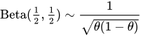
where θ is the vertex variable for the asymmetric triangular distribution with support [0, 1] (corresponding to the following parameter values in Wikipedia's article on the triangular distribution: vertex c = θ, left end a = 0, and right end b = 1). Berger et al. also give a heuristic argument that Beta(1/2,1/2) could indeed be the exact Berger–Bernardo–Sun reference prior for the asymmetric triangular distribution. Therefore, Beta(1/2,1/2) not only is Jeffreys prior for the Bernoulli and binomial distributions, but also seems to be the Berger–Bernardo–Sun reference prior for the asymmetric triangular distribution (for which the Jeffreys prior does not exist), a distribution used in project management and PERT analysis to describe the cost and duration of project tasks.
Clarke and Barron[68] prove that, among continuous positive priors, Jeffreys prior (when it exists) asymptotically maximizes Shannon's mutual information between a sample of size n and the parameter, and therefore Jeffreys prior is the most uninformative prior (measuring information as Shannon information). The proof rests on an examination of the Kullback–Leibler divergence between probability density functions for iid random variables.
Effect of different prior probability choices on the posterior beta distribution
If samples are drawn from the population of a random variable X that result in s successes and f failures in nBernoulli trialsn = s + f, then the likelihood function for parameters s and f given x = p (the notation x = p in the expressions below will emphasize that the domain x stands for the value of the parameter p in the binomial distribution), is the following binomial distribution:

If beliefs about prior probability information are reasonably well approximated by a beta distribution with parameters α Prior and β Prior, then:

According to Bayes' theorem for a continuous event space, the posterior probability density is given by the product of the prior probability and the likelihood function (given the evidence s and f = n − s), normalized so that the area under the curve equals one, as follows:
![{\displaystyle {\begin{aligned}&{\text{posterior probability density}}(x=p\mid s,n-s)\\[6pt]={}&{\frac {\operatorname {priorprobabilitydensity} (x=p;\alpha \operatorname {prior} ,\beta \operatorname {prior} ){\mathcal {L}}(s,f\mid x=p)}{\int _{0}^{1}{\text{prior probability density}}(x=p;\alpha \operatorname {prior} ,\beta \operatorname {prior} ){\mathcal {L}}(s,f\mid x=p)\,dx}}\\[6pt]={}&{\frac {{n \choose s}x^{s+\alpha \operatorname {prior} -1}(1-x)^{n-s+\beta \operatorname {prior} -1}/\mathrm {B} (\alpha \operatorname {prior} ,\beta \operatorname {prior} )}{\int _{0}^{1}\left({n \choose s}x^{s+\alpha \operatorname {prior} -1}(1-x)^{n-s+\beta \operatorname {prior} -1}/\mathrm {B} (\alpha \operatorname {prior} ,\beta \operatorname {prior} )\right)\,dx}}\\[6pt]={}&{\frac {x^{s+\alpha \operatorname {prior} -1}(1-x)^{n-s+\beta \operatorname {prior} -1}}{\int _{0}^{1}\left(x^{s+\alpha \operatorname {prior} -1}(1-x)^{n-s+\beta \operatorname {prior} -1}\right)\,dx}}\\[6pt]={}&{\frac {x^{s+\alpha \operatorname {prior} -1}(1-x)^{n-s+\beta \operatorname {prior} -1}}{\mathrm {B} (s+\alpha \operatorname {prior} ,n-s+\beta \operatorname {prior} )}}.\end{aligned}}}](https://wikimedia.org/api/rest_v1/media/math/render/svg/569ad0317cf545ff98538c8a845f216120e87c08)

appears both in the numerator and the denominator of the posterior probability, and it does not depend on the integration variable x, hence it cancels out, and it is irrelevant to the final result. Similarly the normalizing factor for the prior probability, the beta function B(αPrior,βPrior) cancels out and it is immaterial to the final result. The same posterior probability result can be obtained if one uses an un-normalized prior

because the normalizing factors all cancel out. Several authors (including Jeffreys himself) thus use an un-normalized prior formula since the normalization constant cancels out. The numerator of the posterior probability ends up being just the (un-normalized) product of the prior probability and the likelihood function, and the denominator is its integral from zero to one. The beta function in the denominator, B(s + α Prior, n − s + β Prior), appears as a normalization constant to ensure that the total posterior probability integrates to unity.
The ratio s/n of the number of successes to the total number of trials is a sufficient statistic in the binomial case, which is relevant for the following results.
For the Bayes' prior probability (Beta(1,1)), the posterior probability is:

For the Jeffreys' prior probability (Beta(1/2,1/2)), the posterior probability is:

and for the Haldane prior probability (Beta(0,0)), the posterior probability is:

From the above expressions it follows that for s/n = 1/2) all the above three prior probabilities result in the identical location for the posterior probability mean = mode = 1/2. For s/n < 1/2, the mean of the posterior probabilities, using the following priors, are such that: mean for Bayes prior > mean for Jeffreys prior > mean for Haldane prior. For s/n > 1/2 the order of these inequalities is reversed such that the Haldane prior probability results in the largest posterior mean. The Haldane prior probability Beta(0,0) results in a posterior probability density with mean (the expected value for the probability of success in the "next" trial) identical to the ratio s/n of the number of successes to the total number of trials. Therefore, the Haldane prior results in a posterior probability with expected value in the next trial equal to the maximum likelihood. The Bayes prior probability Beta(1,1) results in a posterior probability density with mode identical to the ratio s/n (the maximum likelihood).
In the case that 100% of the trials have been successful s = n, the Bayes prior probability Beta(1,1) results in a posterior expected value equal to the rule of succession (n + 1)/(n + 2), while the Haldane prior Beta(0,0) results in a posterior expected value of 1 (absolute certainty of success in the next trial). Jeffreys prior probability results in a posterior expected value equal to (n + 1/2)/(n + 1). Perks[62] (p. 303) points out: "This provides a new rule of succession and expresses a 'reasonable' position to take up, namely, that after an unbroken run of n successes we assume a probability for the next trial equivalent to the assumption that we are about half-way through an average run, i.e. that we expect a failure once in (2n + 2) trials. The Bayes–Laplace rule implies that we are about at the end of an average run or that we expect a failure once in (n + 2) trials. The comparison clearly favours the new result (what is now called Jeffreys prior) from the point of view of 'reasonableness'."
Conversely, in the case that 100% of the trials have resulted in failure (s = 0), the Bayes prior probability Beta(1,1) results in a posterior expected value for success in the next trial equal to 1/(n + 2), while the Haldane prior Beta(0,0) results in a posterior expected value of success in the next trial of 0 (absolute certainty of failure in the next trial). Jeffreys prior probability results in a posterior expected value for success in the next trial equal to (1/2)/(n + 1), which Perks[62] (p. 303) points out: "is a much more reasonably remote result than the Bayes–Laplace result 1/(n + 2)".
Jaynes[53] questions (for the Haldane prior Beta(0,0)) the use of these formulas for the cases s = 0 or s = n because the integrals do not converge (Beta(0,0) is an improper prior for s = 0 or s = n). In practice, the conditions 0<s<n necessary for a mode to exist between both ends for the Bayes prior are usually met, and therefore the Bayes prior (as long as 0 < s < n) results in a posterior mode located between both ends of the domain.
As remarked in the section on the rule of succession, K. Pearson showed that after n successes in n trials the posterior probability (based on the Bayes Beta(1,1) distribution as the prior probability) that the next (n + 1) trials will all be successes is exactly 1/2, whatever the value of n. Based on the Haldane Beta(0,0) distribution as the prior probability, this posterior probability is 1 (absolute certainty that after n successes in n trials the next (n + 1) trials will all be successes). Perks[62] (p. 303) shows that, for what is now known as the Jeffreys prior, this probability is ((n + 1/2)/(n + 1))((n + 3/2)/(n + 2))...(2n + 1/2)/(2n + 1), which for n = 1, 2, 3 gives 15/24, 315/480, 9009/13440; rapidly approaching a limiting value of as n tends to infinity. Perks remarks that what is now known as the Jeffreys prior: "is clearly more 'reasonable' than either the Bayes–Laplace result or the result on the (Haldane) alternative rule rejected by Jeffreys which gives certainty as the probability. It clearly provides a very much better correspondence with the process of induction. Whether it is 'absolutely' reasonable for the purpose, i.e. whether it is yet large enough, without the absurdity of reaching unity, is a matter for others to decide. But it must be realized that the result depends on the assumption of complete indifference and absence of knowledge prior to the sampling experiment."

Following are the variances of the posterior distribution obtained with these three prior probability distributions:
for the Bayes' prior probability (Beta(1,1)), the posterior variance is:

for the Jeffreys' prior probability (Beta(1/2,1/2)), the posterior variance is:

and for the Haldane prior probability (Beta(0,0)), the posterior variance is:

So, as remarked by Silvey,[51] for large n, the variance is small and hence the posterior distribution is highly concentrated, whereas the assumed prior distribution was very diffuse. This is in accord with what one would hope for, as vague prior knowledge is transformed (through Bayes' theorem) into a more precise posterior knowledge by an informative experiment. For small n the Haldane Beta(0,0) prior results in the largest posterior variance while the Bayes Beta(1,1) prior results in the more concentrated posterior. Jeffreys prior Beta(1/2,1/2) results in a posterior variance in between the other two. As n increases, the variance rapidly decreases so that the posterior variance for all three priors converges to approximately the same value (approaching zero variance as n → ∞). Recalling the previous result that the Haldane prior probability Beta(0,0) results in a posterior probability density with mean (the expected value for the probability of success in the "next" trial) identical to the ratio s/n of the number of successes to the total number of trials, it follows from the above expression that also the Haldane prior Beta(0,0) results in a posterior with variance identical to the variance expressed in terms of the max. likelihood estimate s/n and sample size (in § Variance):

with the mean μ = s/n and the sample size ν = n.
In Bayesian inference, using a prior distribution Beta(αPrior,βPrior) prior to a binomial distribution is equivalent to adding (αPrior − 1) pseudo-observations of "success" and (βPrior − 1) pseudo-observations of "failure" to the actual number of successes and failures observed, then estimating the parameter p of the binomial distribution by the proportion of successes over both real- and pseudo-observations. A uniform prior Beta(1,1) does not add (or subtract) any pseudo-observations since for Beta(1,1) it follows that (αPrior − 1) = 0 and (βPrior − 1) = 0. The Haldane prior Beta(0,0) subtracts one pseudo observation from each and Jeffreys prior Beta(1/2,1/2) subtracts 1/2 pseudo-observation of success and an equal number of failure. This subtraction has the effect of smoothing out the posterior distribution. If the proportion of successes is not 50% (s/n ≠ 1/2) values of αPrior and βPrior less than 1 (and therefore negative (αPrior − 1) and (βPrior − 1)) favor sparsity, i.e. distributions where the parameter p is closer to either 0 or 1. In effect, values of αPrior and βPrior between 0 and 1, when operating together, function as a concentration parameter.
The accompanying plots show the posterior probability density functions for sample sizes n ∈ {3,10,50}, successes s ∈ {n/2,n/4} and Beta(αPrior,βPrior) ∈ {Beta(0,0),Beta(1/2,1/2),Beta(1,1)}. Also shown are the cases for n = {4,12,40}, success s = {n/4} and Beta(αPrior,βPrior) ∈ {Beta(0,0),Beta(1/2,1/2),Beta(1,1)}. The first plot shows the symmetric cases, for successes s ∈ {n/2}, with mean = mode = 1/2 and the second plot shows the skewed cases s ∈ {n/4}. The images show that there is little difference between the priors for the posterior with sample size of 50 (characterized by a more pronounced peak near p = 1/2). Significant differences appear for very small sample sizes (in particular for the flatter distribution for the degenerate case of sample size = 3). Therefore, the skewed cases, with successes s = {n/4}, show a larger effect from the choice of prior, at small sample size, than the symmetric cases. For symmetric distributions, the Bayes prior Beta(1,1) results in the most "peaky" and highest posterior distributions and the Haldane prior Beta(0,0) results in the flattest and lowest peak distribution. The Jeffreys prior Beta(1/2,1/2) lies in between them. For nearly symmetric, not too skewed distributions the effect of the priors is similar. For very small sample size (in this case for a sample size of 3) and skewed distribution (in this example for s ∈ {n/4}) the Haldane prior can result in a reverse-J-shaped distribution with a singularity at the left end. However, this happens only in degenerate cases (in this example n = 3 and hence s = 3/4 < 1, a degenerate value because s should be greater than unity in order for the posterior of the Haldane prior to have a mode located between the ends, and because s = 3/4 is not an integer number, hence it violates the initial assumption of a binomial distribution for the likelihood) and it is not an issue in generic cases of reasonable sample size (such that the condition 1 < s < n − 1, necessary for a mode to exist between both ends, is fulfilled).
In Chapter 12 (p. 385) of his book, Jaynes[53] asserts that the Haldane prior Beta(0,0) describes a prior state of knowledge of complete ignorance, where we are not even sure whether it is physically possible for an experiment to yield either a success or a failure, while the Bayes (uniform) prior Beta(1,1) applies if one knows that both binary outcomes are possible. Jaynes states: "interpret the Bayes–Laplace (Beta(1,1)) prior as describing not a state of complete ignorance, but the state of knowledge in which we have observed one success and one failure...once we have seen at least one success and one failure, then we know that the experiment is a true binary one, in the sense of physical possibility." Jaynes [53] does not specifically discuss Jeffreys prior Beta(1/2,1/2) (Jaynes discussion of "Jeffreys prior" on pp. 181, 423 and on chapter 12 of Jaynes book[53] refers instead to the improper, un-normalized, prior "1/p dp" introduced by Jeffreys in the 1939 edition of his book,[60] seven years before he introduced what is now known as Jeffreys' invariant prior: the square root of the determinant of Fisher's information matrix. "1/p" is Jeffreys' (1946) invariant prior for the exponential distribution, not for the Bernoulli or binomial distributions). However, it follows from the above discussion that Jeffreys Beta(1/2,1/2) prior represents a state of knowledge in between the Haldane Beta(0,0) and Bayes Beta (1,1) prior.
Similarly, Karl Pearson in his 1892 book The Grammar of Science[69][70] (p. 144 of 1900 edition) maintained that the Bayes (Beta(1,1) uniform prior was not a complete ignorance prior, and that it should be used when prior information justified to "distribute our ignorance equally"". K. Pearson wrote: "Yet the only supposition that we appear to have made is this: that, knowing nothing of nature, routine and anomy (from the Greek ανομία, namely: a- "without", and nomos "law") are to be considered as equally likely to occur. Now we were not really justified in making even this assumption, for it involves a knowledge that we do not possess regarding nature. We use our experience of the constitution and action of coins in general to assert that heads and tails are equally probable, but we have no right to assert before experience that, as we know nothing of nature, routine and breach are equally probable. In our ignorance we ought to consider before experience that nature may consist of all routines, all anomies (normlessness), or a mixture of the two in any proportion whatever, and that all such are equally probable. Which of these constitutions after experience is the most probable must clearly depend on what that experience has been like."
If there is sufficient sampling data, and the posterior probability mode is not located at one of the extremes of the domain (x = 0 or x = 1), the three priors of Bayes (Beta(1,1)), Jeffreys (Beta(1/2,1/2)) and Haldane (Beta(0,0)) should yield similar posterior probability densities. Otherwise, as Gelman et al.[71] (p. 65) point out, "if so few data are available that the choice of noninformative prior distribution makes a difference, one should put relevant information into the prior distribution", or as Berger[4] (p. 125) points out "when different reasonable priors yield substantially different answers, can it be right to state that there is a single answer? Would it not be better to admit that there is scientific uncertainty, with the conclusion depending on prior beliefs?."
Occurrence and applications
Order statistics
The beta distribution has an important application in the theory of order statistics. A basic result is that the distribution of the kth smallest of a sample of size n from a continuous uniform distribution has a beta distribution.[40] This result is summarized as

From this, and application of the theory related to the probability integral transform, the distribution of any individual order statistic from any continuous distribution can be derived.[40]
Subjective logic
In standard logic, propositions are considered to be either true or false. In contradistinction, subjective logic assumes that humans cannot determine with absolute certainty whether a proposition about the real world is absolutely true or false. In subjective logic the posteriori probability estimates of binary events can be represented by beta distributions.[72]
Wavelet analysis
A wavelet is a wave-like oscillation with an amplitude that starts out at zero, increases, and then decreases back to zero. It can typically be visualized as a "brief oscillation" that promptly decays. Wavelets can be used to extract information from many different kinds of data, including – but certainly not limited to – audio signals and images. Thus, wavelets are purposefully crafted to have specific properties that make them useful for signal processing. Wavelets are localized in both time and frequency whereas the standard Fourier transform is only localized in frequency. Therefore, standard Fourier Transforms are only applicable to stationary processes, while wavelets are applicable to non-stationary processes. Continuous wavelets can be constructed based on the beta distribution. Beta wavelets[73] can be viewed as a soft variety of Haar wavelets whose shape is fine-tuned by two shape parameters α and β.
Population genetics
The Balding–Nichols model is a two-parameter parametrization of the beta distribution used in population genetics.[74] It is a statistical description of the allele frequencies in the components of a sub-divided population:
where and ; here F is (Wright's) genetic distance between two populations.
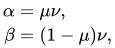
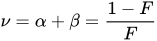

Project management: task cost and schedule modeling
The beta distribution can be used to model events which are constrained to take place within an interval defined by a minimum and maximum value. For this reason, the beta distribution — along with the triangular distribution — is used extensively in PERT, critical path method (CPM), Joint Cost Schedule Modeling (JCSM) and other project management/control systems to describe the time to completion and the cost of a task. In project management, shorthand computations are widely used to estimate the mean and standard deviation of the beta distribution:[39]
![{\displaystyle {\begin{aligned}\mu (X)&={\frac {a+4b+c}{6}}\\[8pt]\sigma (X)&={\frac {c-a}{6}}\end{aligned}}}](https://wikimedia.org/api/rest_v1/media/math/render/svg/7a89a68d1250ebe659be15e88edb5a9eb3e0cf87)
where a is the minimum, c is the maximum, and b is the most likely value (the mode for α > 1 and β > 1).
The above estimate for the mean is known as the PERTthree-point estimation and it is exact for either of the following values of β (for arbitrary α within these ranges):
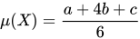
- β = α > 1 (symmetric case) with standard deviation, skewness = 0, and excess kurtosis =
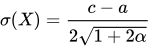


or
- β = 6 − α for 5 > α > 1 (skewed case) with standard deviation
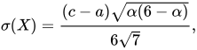
skewness, and excess kurtosis
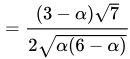
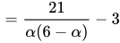

The above estimate for the standard deviationσ(X) = (c − a)/6 is exact for either of the following values of α and β:
- α = β = 4 (symmetric) with skewness = 0, and excess kurtosis = −6/11.
- β = 6 − α and (right-tailed, positive skew) with skewness, and excess kurtosis = 0
- β = 6 − α and (left-tailed, negative skew) with skewness, and excess kurtosis = 0


Otherwise, these can be poor approximations for beta distributions with other values of α and β, exhibiting average errors of 40% in the mean and 549% in the variance.[75][76][77]
Random variate generation
If X and Y are independent, with and then


So one algorithm for generating beta variates is to generate , where X is a gamma variate with parameters (α, 1) and Y is an independent gamma variate with parameters (β, 1).[78] In fact, here and are independent, and . If and is independent of and , then and is independent of . This shows that the product of independent and random variables is a random variable.





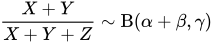


Also, the kth order statistic of nuniformly distributed variates is , so an alternative if α and β are small integers is to generate α + β − 1 uniform variates and choose the α-th smallest.[40]

Another way to generate the Beta distribution is by Pólya urn model. According to this method, one starts with an "urn" with α "black" balls and β "white" balls and draws uniformly with replacement. Every trial an additional ball is added according to the color of the last ball which was drawn. Asymptotically, the proportion of black and white balls will be distributed according to the Beta distribution, where each repetition of the experiment will produce a different value.
It is also possible to use the inverse transform sampling.
Normal approximation to the Beta distribution
A beta distribution with and and is approximately normal with mean and variance . If the normal approximation can be improved by taking the cube-root of the logarithm of the reciprocal of [79][80]


History
Thomas Bayes, in a posthumous paper [63] published in 1763 by Richard Price, obtained a beta distribution as the density of the probability of success in Bernoulli trials (see § Applications, Bayesian inference), but the paper does not analyze any of the moments of the beta distribution or discuss any of its properties.
The first systematic modern discussion of the beta distribution is probably due to Karl Pearson.[81][82] In Pearson's papers[21][33] the beta distribution is couched as a solution of a differential equation: Pearson's Type I distribution which it is essentially identical to except for arbitrary shifting and re-scaling (the beta and Pearson Type I distributions can always be equalized by proper choice of parameters). In fact, in several English books and journal articles in the few decades prior to World War II, it was common to refer to the beta distribution as Pearson's Type I distribution. William P. Elderton in his 1906 monograph "Frequency curves and correlation"[43] further analyzes the beta distribution as Pearson's Type I distribution, including a full discussion of the method of moments for the four parameter case, and diagrams of (what Elderton describes as) U-shaped, J-shaped, twisted J-shaped, "cocked-hat" shapes, horizontal and angled straight-line cases. Elderton wrote "I am chiefly indebted to Professor Pearson, but the indebtedness is of a kind for which it is impossible to offer formal thanks." Elderton in his 1906 monograph [43] provides an impressive amount of information on the beta distribution, including equations for the origin of the distribution chosen to be the mode, as well as for other Pearson distributions: types I through VII. Elderton also included a number of appendixes, including one appendix ("II") on the beta and gamma functions. In later editions, Elderton added equations for the origin of the distribution chosen to be the mean, and analysis of Pearson distributions VIII through XII.
As remarked by Bowman and Shenton[45] "Fisher and Pearson had a difference of opinion in the approach to (parameter) estimation, in particular relating to (Pearson's method of) moments and (Fisher's method of) maximum likelihood in the case of the Beta distribution." Also according to Bowman and Shenton, "the case of a Type I (beta distribution) model being the center of the controversy was pure serendipity. A more difficult model of 4 parameters would have been hard to find." The long running public conflict of Fisher with Karl Pearson can be followed in a number of articles in prestigious journals. For example, concerning the estimation of the four parameters for the beta distribution, and Fisher's criticism of Pearson's method of moments as being arbitrary, see Pearson's article "Method of moments and method of maximum likelihood" [46] (published three years after his retirement from University College, London, where his position had been divided between Fisher and Pearson's son Egon) in which Pearson writes "I read (Koshai's paper in the Journal of the Royal Statistical Society, 1933) which as far as I am aware is the only case at present published of the application of Professor Fisher's method. To my astonishment that method depends on first working out the constants of the frequency curve by the (Pearson) Method of Moments and then superposing on it, by what Fisher terms "the Method of Maximum Likelihood" a further approximation to obtain, what he holds, he will thus get, 'more efficient values' of the curve constants".
David and Edwards's treatise on the history of statistics[83] cites the first modern treatment of the beta distribution, in 1911,[84] using the beta designation that has become standard, due to Corrado Gini, an Italian statistician, demographer, and sociologist, who developed the Gini coefficient. N.L.Johnson and S.Kotz, in their comprehensive and very informative monograph[85] on leading historical personalities in statistical sciences credit Corrado Gini[86] as "an early Bayesian...who dealt with the problem of eliciting the parameters of an initial Beta distribution, by singling out techniques which anticipated the advent of the so-called empirical Bayes approach."
References
- 12345678910111213141516171819202122232425Johnson, Norman L.; Kotz, Samuel; Balakrishnan, N. (1995). "Chapter 25: Beta Distributions". Continuous Univariate Distributions Vol. 2 (2nd ed.). Wiley. ISBN 978-0-471-58494-0.
- 12Rose, Colin; Smith, Murray D. (2002). Mathematical Statistics with MATHEMATICA. Springer. ISBN 978-0387952345.
- 123Kruschke, John K. (2011). Doing Bayesian data analysis: A tutorial with R and BUGS. Academic Press / Elsevier. p. 83. ISBN 978-0123814852.
- 12Berger, James O. (2010). Statistical Decision Theory and Bayesian Analysis (2nd ed.). Springer. ISBN 978-1441930743.
- 123Feller, William (1971). An Introduction to Probability Theory and Its Applications, Vol. 2. Wiley. ISBN 978-0471257097.
- ↑Wadsworth, G. P. (1960). Introduction to Probability and Random Variables. New York: McGraw-Hill. p. 52.
- ↑Kruschke, John K. (2015). Doing Bayesian Data Analysis: A Tutorial with R, JAGS and Stan. Academic Press / Elsevier. ISBN 978-0-12-405888-0.
- 12Wadsworth, George P. and Joseph Bryan (1960). Introduction to Probability and Random Variables. McGraw-Hill.
- 1234567Gupta, Arjun K., ed. (2004). Handbook of Beta Distribution and Its Applications. CRC Press. ISBN 978-0824753962.
- 12Kerman, Jouni (2011). "A closed-form approximation for the median of the beta distribution". arXiv:1111.0433 [math.ST].
- ↑Mosteller, Frederick and John Tukey (1977). Data Analysis and Regression: A Second Course in Statistics. Addison-Wesley Pub. Co. Bibcode:1977dars.book.....M. ISBN 978-0201048544.
- ↑Feller, William (1968). An Introduction to Probability Theory and Its Applications. Vol. 1 (3rd ed.). Wiley. ISBN 978-0471257080.
- ↑Philip J. Fleming and John J. Wallace. How not to lie with statistics: the correct way to summarize benchmark results. Communications of the ACM, 29(3):218–221, March 1986.
- ↑"NIST/SEMATECH e-Handbook of Statistical Methods 1.3.6.6.17. Beta Distribution". National Institute of Standards and Technology Information Technology Laboratory. April 2012. Retrieved May 31, 2016.
- ↑Oguamanam, D.C.D.; Martin, H. R.; Huissoon, J. P. (1995). "On the application of the beta distribution to gear damage analysis". Applied Acoustics. 45 (3): 247–261. doi:10.1016/0003-682X(95)00001-P.
- ↑Zhiqiang Liang; Jianming Wei; Junyu Zhao; Haitao Liu; Baoqing Li; Jie Shen; Chunlei Zheng (27 August 2008). "The Statistical Meaning of Kurtosis and Its New Application to Identification of Persons Based on Seismic Signals". Sensors. 8 (8): 5106–5119. Bibcode:2008Senso...8.5106L. doi:10.3390/s8085106. PMC 3705491. PMID 27873804.
- ↑Kenney, J. F., and E. S. Keeping (1951). Mathematics of Statistics Part Two, 2nd edition. D. Van Nostrand Company Inc.
{{cite book}}: CS1 maint: multiple names: authors list (link) - 1234Abramowitz, Milton and Irene A. Stegun (1965). Handbook Of Mathematical Functions With Formulas, Graphs, And Mathematical Tables. Dover. ISBN 978-0-486-61272-0.
- ↑Weisstein., Eric W. "Kurtosis". MathWorld--A Wolfram Web Resource. Retrieved 13 August 2012.
- 12Panik, Michael J (2005). Advanced Statistics from an Elementary Point of View. Academic Press. ISBN 978-0120884940.
- 123456Pearson, Karl (1916). "Mathematical contributions to the theory of evolution, XIX: Second supplement to a memoir on skew variation". Philosophical Transactions of the Royal Society A. 216 (538–548): 429–457. Bibcode:1916RSPTA.216..429P. doi:10.1098/rsta.1916.0009. JSTOR 91092.
- ↑Gradshteyn, Izrail Solomonovich; Ryzhik, Iosif Moiseevich; Geronimus, Yuri Veniaminovich; Tseytlin, Michail Yulyevich; Jeffrey, Alan (2015) [October 2014]. Zwillinger, Daniel; Moll, Victor Hugo (eds.). Table of Integrals, Series, and Products. Translated by Scripta Technica, Inc. (8 ed.). Academic Press, Inc.ISBN 978-0-12-384933-5. LCCN 2014010276.
- ↑Billingsley, Patrick (1995). "Section 30: The Method of Moments". Probability and measure (3rd ed.). Wiley-Interscience. ISBN 978-0-471-00710-4.
- 12MacKay, David (2003). Information Theory, Inference and Learning Algorithms. Cambridge University Press; First Edition. Bibcode:2003itil.book.....M. ISBN 978-0521642989.
- 12Johnson, N.L. (1949). "Systems of frequency curves generated by methods of translation"(PDF). Biometrika. 36 (1–2): 149–176. doi:10.1093/biomet/36.1-2.149. hdl:10338.dmlcz/135506. PMID 18132090.
- ↑Verdugo Lazo, A. C. G.; Rathie, P. N. (1978). "On the entropy of continuous probability distributions". IEEE Trans. Inf. Theory. 24 (1): 120–122. doi:10.1109/TIT.1978.1055832.
- ↑Shannon, Claude E. (1948). "A Mathematical Theory of Communication". Bell System Technical Journal. 27 (4): 623–656. doi:10.1002/j.1538-7305.1948.tb01338.x.
- 123Cover, Thomas M. and Joy A. Thomas (2006). Elements of Information Theory 2nd Edition (Wiley Series in Telecommunications and Signal Processing). Wiley-Interscience; 2 edition. ISBN 978-0471241959.
- ↑Plunkett, Kim, and Jeffrey Elman (1997). Exercises in Rethinking Innateness: A Handbook for Connectionist Simulations (Neural Network Modeling and Connectionism). A Bradford Book. p. 166. ISBN 978-0262661058.
{{cite book}}: CS1 maint: multiple names: authors list (link) - ↑Nallapati, Ramesh (2006). The smoothed dirichlet distribution: understanding cross-entropy ranking in information retrieval (Thesis). Computer Science Dept., University of Massachusetts Amherst.
- 12Pearson, Egon S. (July 1969). "Some historical reflections traced through the development of the use of frequency curves". THEMIS Statistical Analysis Research Program, Technical Report 38. Office of Naval Research, Contract N000014-68-A-0515 (Project NR 042–260).
- ↑Hahn, Gerald J.; Shapiro, S. (1994). Statistical Models in Engineering (Wiley Classics Library). Wiley-Interscience. ISBN 978-0471040651.
- 12Pearson, Karl (1895). "Contributions to the mathematical theory of evolution, II: Skew variation in homogeneous material". Philosophical Transactions of the Royal Society. 186: 343–414. Bibcode:1895RSPTA.186..343P. doi:10.1098/rsta.1895.0010. JSTOR 90649.
- ↑Buchanan, K.; Rockway, J.; Sternberg, O.; Mai, N. N. (May 2016). "Sum-difference beamforming for radar applications using circularly tapered random arrays". 2016 IEEE Radar Conference (RadarConf). pp. 1–5. doi:10.1109/RADAR.2016.7485289. ISBN 978-1-5090-0863-6. S2CID 32525626.
- ↑Buchanan, K.; Flores, C.; Wheeland, S.; Jensen, J.; Grayson, D.; Huff, G. (May 2017). "Transmit beamforming for radar applications using circularly tapered random arrays". 2017 IEEE Radar Conference (RadarConf). pp. 0112–0117. doi:10.1109/RADAR.2017.7944181. ISBN 978-1-4673-8823-8. S2CID 38429370.
- ↑Ryan, Buchanan, Kristopher (2014-05-29). "Theory and Applications of Aperiodic (Random) Phased Arrays".
{{cite web}}: CS1 maint: multiple names: authors list (link) - ↑Pham-Gia, T. (January 2000). "Distributions of the ratios of independent beta variables and applications". Communications in Statistics - Theory and Methods. 29 (12): 2693–2715. doi:10.1080/03610920008832632. ISSN 0361-0926. Retrieved 13 November 2024.
- ↑Herrerías-Velasco, José Manuel and Herrerías-Pleguezuelo, Rafael and René van Dorp, Johan. (2011). Revisiting the PERT mean and Variance. European Journal of Operational Research (210), p. 448–451.
- 12Malcolm, D. G.; Roseboom, J. H.; Clark, C. E.; Fazar, W. (September–October 1958). "Application of a Technique for Research and Development Program Evaluation". Operations Research. 7 (5): 646–669. doi:10.1287/opre.7.5.646. ISSN 0030-364X.
- 1234David, H. A., Nagaraja, H. N. (2003) Order Statistics (3rd Edition). Wiley, New Jersey pp 458. ISBN 0-471-38926-9
- ↑Lee, Changwoo J.; Zito, Alessandro; Sang, Huiyan; Dunson, David B. (2025-12-01). "Logistic-Beta Processes for Dependent Random Probabilities with Beta Marginals". Bayesian Analysis. 20 (4). doi:10.1214/25-ba1541. ISSN 1936-0975.
- ↑"1.3.6.6.17. Beta Distribution". www.itl.nist.gov.
- 12345678Elderton, William Palin (1906). Frequency-Curves and Correlation. Charles and Edwin Layton (London).
- ↑Elderton, William Palin and Norman Lloyd Johnson (2009). Systems of Frequency Curves. Cambridge University Press. ISBN 978-0521093361.
- 123Bowman, K. O.; Shenton, L. R. (2007). "The beta distribution, moment method, Karl Pearson and R.A. Fisher"(PDF). Far East J. Theo. Stat. 23 (2): 133–164.
- 12Pearson, Karl (June 1936). "Method of moments and method of maximum likelihood". Biometrika. 28 (1/2): 34–59. doi:10.2307/2334123. JSTOR 2334123.
- 123Joanes, D. N.; C. A. Gill (1998). "Comparing measures of sample skewness and kurtosis". The Statistician. 47 (Part 1): 183–189. doi:10.1111/1467-9884.00122.
- ↑Beckman, R. J.; G. L. Tietjen (1978). "Maximum likelihood estimation for the beta distribution". Journal of Statistical Computation and Simulation. 7 (3–4): 253–258. doi:10.1080/00949657808810232.
- ↑Gnanadesikan, R., Pinkham and Hughes (1967). "Maximum likelihood estimation of the parameters of the beta distribution from smallest order statistics". Technometrics. 9 (4): 607–620. doi:10.2307/1266199. JSTOR 1266199.
{{cite journal}}: CS1 maint: multiple names: authors list (link) - ↑Fackler, Paul. "Inverse Digamma Function (Matlab)". Harvard University School of Engineering and Applied Sciences. Retrieved 2012-08-18.
- 123Silvey, S.D. (1975). Statistical Inference. Chapman and Hal. p. 40. ISBN 978-0412138201.
- ↑Edwards, A. W. F. (1992). Likelihood. The Johns Hopkins University Press. ISBN 978-0801844430.
- 123456Jaynes, E.T. (2003). Probability theory, the logic of science. Cambridge University Press. ISBN 978-0521592710.
- ↑Costa, Max, and Cover, Thomas (September 1983). On the similarity of the entropy power inequality and the Brunn Minkowski inequality(PDF). Tech.Report 48, Dept. Statistics, Stanford University.
{{cite book}}: CS1 maint: multiple names: authors list (link) - 123Aryal, Gokarna; Saralees Nadarajah (2004). "Information matrix for beta distributions"(PDF). Serdica Mathematical Journal (Bulgarian Academy of Science). 30: 513–526.
- 12Laplace, Pierre Simon, marquis de (1902). A philosophical essay on probabilities. New York : J. Wiley; London : Chapman & Hall. ISBN 978-1-60206-328-0.
{{cite book}}: ISBN / Date incompatibility (help)CS1 maint: multiple names: authors list (link) - ↑Cox, Richard T. (1961). Algebra of Probable Inference. The Johns Hopkins University Press. ISBN 978-0801869822.
{{cite book}}: ISBN / Date incompatibility (help) - 12Keynes, John Maynard (2010) [1921]. A Treatise on Probability: The Connection Between Philosophy and the History of Science. Wildside Press. ISBN 978-1434406965.
- ↑Pearson, Karl (1907). "On the Influence of Past Experience on Future Expectation". Philosophical Magazine. 6 (13): 365–378.
- 1234Jeffreys, Harold (1998). Theory of Probability. Oxford University Press, 3rd edition. ISBN 978-0198503682.
- ↑Broad, C. D. (October 1918). "On the relation between induction and probability". MIND, A Quarterly Review of Psychology and Philosophy. 27 (New Series) (108): 389–404. doi:10.1093/mind/XXVII.4.389. JSTOR 2249035.
- 1234Perks, Wilfred (January 1947). "Some observations on inverse probability including a new indifference rule". Journal of the Institute of Actuaries. 73 (2): 285–334. doi:10.1017/S0020268100012270. Archived from the original on 2014-01-12. Retrieved 2012-09-19.
- 12Bayes, Thomas; communicated by Richard Price (1763). "An Essay towards solving a Problem in the Doctrine of Chances". Philosophical Transactions of the Royal Society. 53: 370–418. doi:10.1098/rstl.1763.0053. JSTOR 105741.
- ↑Haldane, J. B. S. (1932). "A note on inverse probability". Mathematical Proceedings of the Cambridge Philosophical Society. 28 (1): 55–61. Bibcode:1932PCPS...28...55H. doi:10.1017/s0305004100010495. S2CID 122773707.
- ↑Zellner, Arnold (1971). An Introduction to Bayesian Inference in Econometrics. Wiley-Interscience. ISBN 978-0471169376.
- ↑Jeffreys, Harold (September 1946). "An Invariant Form for the Prior Probability in Estimation Problems". Proceedings of the Royal Society. A 24. 186 (1007): 453–461. Bibcode:1946RSPSA.186..453J. doi:10.1098/rspa.1946.0056. PMID 20998741.
- ↑Berger, James; Bernardo, Jose; Sun, Dongchu (2009). "The formal definition of reference priors". The Annals of Statistics. 37 (2): 905–938. arXiv:0904.0156. Bibcode:2009arXiv0904.0156B. doi:10.1214/07-AOS587. S2CID 3221355.
- ↑Clarke, Bertrand S.; Andrew R. Barron (1994). "Jeffreys' prior is asymptotically least favorable under entropy risk"(PDF). Journal of Statistical Planning and Inference. 41: 37–60. doi:10.1016/0378-3758(94)90153-8.
- ↑Pearson, Karl (1892). The Grammar of Science. Walter Scott, London.
- ↑Pearson, Karl (2009). The Grammar of Science. BiblioLife. ISBN 978-1110356119.
- ↑Gelman, A., Carlin, J. B., Stern, H. S., and Rubin, D. B. (2003). Bayesian Data Analysis. Chapman and Hall/CRC. ISBN 978-1584883883.
{{cite book}}: CS1 maint: multiple names: authors list (link) - ↑Jøsang, Audun (2001). "A logic for uncertain probabilities". International Journal of Uncertainty, Fuzziness and Knowledge-Based Systems. 9 (3): 279–311. doi:10.1142/S0218488501000831. MR 1843261.
- ↑H.M. de Oliveira and G.A.A. Araújo,. Compactly Supported One-cyclic Wavelets Derived from Beta Distributions. Journal of Communication and Information Systems. vol.20, n.3, pp.27-33, 2005.
- ↑Balding, David J.; Nichols, Richard A. (1995). "A method for quantifying differentiation between populations at multi-allelic loci and its implications for investigating identity and paternity". Genetica. 96 (1–2). Springer: 3–12. doi:10.1007/BF01441146. PMID 7607457. S2CID 30680826.
- ↑Keefer, Donald L. and Verdini, William A. (1993). Better Estimation of PERT Activity Time Parameters. Management Science 39(9), p. 1086–1091.
- ↑Keefer, Donald L. and Bodily, Samuel E. (1983). Three-point Approximations for Continuous Random variables. Management Science 29(5), p. 595–609.
- ↑"Defense Resource Management Institute - Naval Postgraduate School". www.nps.edu.
- ↑van der Waerden, Bartel Leendert (1969). Mathematical Statistics. Springer. ISBN 978-3-540-04507-6.
- ↑On normalizing the incomplete beta-function for fitting to dose-response curves M.E. Wise Biometrika vol 47, No. 1/2, June 1960, pp. 173–175
- ↑Pratt, John W. “A Normal Approximation for Binomial, F, Beta, and Other Common, Related Tail Probabilities, II.” Journal of the American Statistical Association, vol. 63, no. 324, 1968, pp. 1457–83. JSTOR, https://doi.org/10.2307/2285896. Accessed 21 Oct. 2025.
- ↑Yule, G. U.; Filon, L. N. G. (1936). "Karl Pearson. 1857–1936". Obituary Notices of Fellows of the Royal Society. 2 (5): 72. doi:10.1098/rsbm.1936.0007. JSTOR 769130.
- ↑"Library and Archive catalogue". Sackler Digital Archive. Royal Society. Archived from the original on 2011-10-25. Retrieved 2011-07-01.
- ↑David, H. A. and A.W.F. Edwards (2001). Annotated Readings in the History of Statistics. Springer; 1 edition. ISBN 978-0387988443.
- ↑Gini, Corrado (1911). "Considerazioni Sulle Probabilità Posteriori e Applicazioni al Rapporto dei Sessi Nelle Nascite Umane". Studi Economico-Giuridici della Università de Cagliari. Anno III (reproduced in Metron 15, 133, 171, 1949): 5–41.
- ↑ جونسون، نورمان ل. وصموئيل كوتز، محرران (1997). شخصيات رائدة في العلوم الإحصائية: من القرن السابع عشر إلى الوقت الحاضر (سلسلة وايلي في الاحتمالات والإحصاء . وايلي. ISBN 978-0471163817.
- ↑ مجلة ميترون. "سيرة كورادو جيني" . مجلة ميترون. مؤرشفة من الأصل بتاريخ 16 يوليو 2012. تم الاطلاع عليها بتاريخ 18 أغسطس 2012 .
روابط خارجية
- "توزيع بيتا" بقلم فيونا ماكلاشلان، مشروع عروض وولفرام ، 2007.
- توزيع بيتا - نظرة عامة ومثال ، xycoon.com
- توزيع النسخة التجريبية ، brighton-webs.co.uk
- فيديو توزيع النسخة التجريبية ، exstrom.com
- "توزيع بيتا" ، موسوعة الرياضيات ، دار نشر EMS ، 2001 [1994]
- وايسشتاين، إريك دبليو. "توزيع بيتا" . عالم الرياضيات .
- جامعة هارفارد، إحصاءات 110، المحاضرة 23: توزيع بيتا، الأستاذ جو بليتزستين
- التوزيعات المستمرة
- موضوعات المضروب والثنائي
- التوزيعات الاحتمالية المترافقة
- توزيعات العائلة الأسية