Binomial sum variance inequality

We wish to prove that

${\displaystyle Var(Z)\leqslant E[Z](1-{\frac {E[Z]}{m_{0}+m_{1}}})}$

We will prove this inequality by finding an expression for Var(Z) and substituting it on the left-hand side, then showing that the inequality always holds.

إذا كان المتغير العشوائي Z يتبع التوزيع الثنائي بمعاملات n و p ، فإن القيمة المتوقعة لـ Z تُعطى بالعلاقة E[ Z ] = np، _وتباين Z يُعطى بالعلاقة Var[ Z ] = np (1 – p ). وبفرض n = m₀ + m₁ _، وبالتعويض عن np بالعلاقة E[ Z ] نحصل على

${\displaystyle Var(Z)=E[Z](1-{\frac {E[Z]}{m_{0}+m_{1}}})}$

المتغيران العشوائيان X و Y مستقلان، لذا فإن تباين المجموع يساوي مجموع التباينات ، أي

${\displaystyle Var(Z)=E[X](1-{\frac {E[X]}{m_{0}}})+E[Y](1-{\frac {E[Y]}{m_{1}}})}$

لإثبات النظرية، يكفي إثبات أن

${\displaystyle E[X](1-{\frac {E[X]}{m_{0}}})+E[Y](1-{\frac {E[Y]}{m_{1}}})\leqslant E[Z](1-{\frac {E[Z]}{m_{0}+m_{1}}})}$

باستبدال E[ X ] + E[ Y ] بـ E[ Z ] نحصل على

${\displaystyle E[X](1-{\frac {E[X]}{m_{0}}})+E[Y](1-{\frac {E[Y]}{m_{1}}})\leqslant (E[X]+E[Y])(1-{\frac {E[X]+E[Y]}{m_{0}+m_{1}}})}$

بضرب الأقواس وطرح E[X] + E[Y] من كلا الطرفين نحصل على:

${\displaystyle -{\frac {E[X]^{2}}{m_{0}}}-{\frac {E[Y]^{2}}{m_{1}}}\leqslant -{\frac {(E[X]+E[Y])^{2}}{m_{0}+m_{1}}}}$

بضرب الأقواس نحصل على

${\displaystyle E[X]-{\frac {E[X]^{2}}{m_{0}}}+E[Y]-{\frac {E[Y]^{2}}{m_{1}}}\leqslant E[X]+E[Y]-{\frac {(E[X]+E[Y])^{2}}{m_{0}+m_{1}}}}$

بطرح E[X] و E[Y] من كلا الطرفين وعكس المتباينة نحصل على

${\displaystyle {\frac {E[X]^{2}}{m_{0}}}+{\frac {E[Y]^{2}}{m_{1}}}\geqslant {\frac {(E[X]+E[Y])^{2}}{m_{0}+m_{1}}}}$

يؤدي توسيع الجانب الأيمن إلى

${\displaystyle {\frac {E[X]^{2}}{m_{0}}}+{\frac {E[Y]^{2}}{m_{1}}}\geqslant {\frac {E[X]^{2}+2E[X]E[Y]+E[Y]^{2}}{m_{0}+m_{1}}}}$

الضرب في${\displaystyle m_{0}m_{1}(m_{0}+m_{1})}$العائد

${\displaystyle (m_{0}m_{1}+{m_{1}}^{2}){E[X]^{2}}+({m_{0}}^{2}+m_{0}m_{1}){E[Y]^{2}}\geqslant m_{0}m_{1}({E[X]}^{2}+2E[X]E[Y]+{E[Y]]^{2}})}$

بطرح الطرف الأيمن نحصل على العلاقة

${\displaystyle {m_{1}}^{2}{E[X]^{2}}-2m_{0}m_{1}E[X]E[Y]+{m_{0}}^{2}{E[Y]^{2}}\geqslant 0}$

أو ما يعادل ذلك

${\displaystyle (m_{1}E[X]-m_{0}E[Y])^{2}\geqslant 0}$

مربع أي عدد حقيقي يكون دائمًا أكبر من أو يساوي الصفر، لذا فإن هذا ينطبق على جميع التوزيعات الثنائية المستقلة التي يمكن أن تأخذها المتغيرات X و Y. وهذا يكفي لإثبات النظرية.

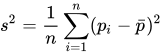
على الرغم من أن هذا البرهان قد طُوِّر لمجموع متغيرين، إلا أنه يُمكن تعميمه بسهولة ليشمل أكثر من متغيرين. إضافةً إلى ذلك، إذا كانت احتمالات النجاح الفردية معروفة، فإن التباين يكون معروفًا بأنه يأخذ الشكل ^{[ 6 ].}

${\displaystyle \operatorname {Var} (Z)=n{\bar {p}}(1- {\bar {p}})-ns^{2},}$

أين${\displaystyle {\bar {p}}}$هو متوسط ​​الاحتمال و${\displaystyle s^{2}={\frac {1}{n}}\sum _{i=1}^{n}(p_{i}-{\bar {p}})^{2}}$يشير هذا التعبير أيضًا إلى أن التباين يكون دائمًا أقل من تباين التوزيع ذي الحدين.${\displaystyle p={\bar {p}}}$، لأن التعبير القياسي للتباين ينخفض ​​بمقدار ns ² ، وهو عدد موجب.

References

- ↑Butler, Ken; Stephens, Michael (1993). "The distribution of a sum of binomial random variables"(PDF). Technical Report No. 467. Department of Statistics, Stanford University. Archived(PDF) from the original on April 11, 2021.
- ↑Nedelman, J and Wallenius, T., 1986. Bernoulli trials, Poisson trials, surprising variances, and Jensen’s Inequality. The American Statistician, 40(4):286–289.
- ↑Feller, W. 1968. An introduction to probability theory and its applications (Vol. 1, 3rd ed.). New York: John Wiley.
- ↑Johnson, N. L. and Kotz, S. 1969. Discrete distributions. New York: John Wiley
- ↑Kendall, M. and Stuart, A. 1977. The advanced theory of statistics. New York: Macmillan.
- 12Drezner, Zvi; Farnum, Nicholas (1993). "A generalized binomial distribution". Communications in Statistics - Theory and Methods. 22 (11): 3051–3063. doi:10.1080/03610929308831202. ISSN 0361-0926.
- ↑Hoeffding, W. 1956. On the distribution of the number of successes in independent trials. Annals of Mathematical Statistics (27):713–721.
- ↑Millstein, J.; Volfson, D. (2013). "Computationally efficient permutation-based confidence interval estimation for tail-area FDR". Frontiers in Genetics. 4 (179): 1–11. doi:10.3389/fgene.2013.00179. PMC 3775454. PMID 24062767.
- Theorems in probability theory
- Theorems in statistics
- Statistical inequalities