
Residual neural network
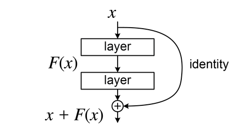
A residual neural network (also referred to as a residual network or ResNet)[1] is a deep learning architecture in which the layers learn residual functions with reference to the layer inputs. It was developed in 2015 for image recognition, and won the ImageNet Large Scale Visual Recognition Challenge (ILSVRC) of that year.[2][3]
As a point of terminology, "residual connection" refers to the specific architectural motif of , where is an arbitrary neural network module. The motif had been used previously (see §History for details). However, the publication of ResNet made it widely popular for feedforward networks, appearing in neural networks that are seemingly unrelated to ResNet.


The residual connection stabilizes the training and convergence of deep neural networks with hundreds of layers, and is a common motif in deep neural networks, such as transformer models (e.g., BERT, and GPT models such as ChatGPT), the AlphaGo Zero system, the AlphaStar system, and the AlphaFold system.
Mathematics
Residual connection
In a multilayer neural network model, consider a (non-residual) subnetwork with a certain number of stacked layers (e.g., 2 or 3). Let denote the subnetwork. Suppose is the desired optimal output of this subnetwork. Residual learning simply adds directly to the output, such that the optimal learned output now becomes , which is interpreted as a "residual" with respect to .


The operation of "adding " is implemented via a "skip connection" that performs an identity mapping to connect the input of the subnetwork with its output. This connection is referred to as a "residual connection" in later work.
Let . The function is often represented by matrix multiplication interlaced with activation functions and normalization operations (e.g., batch normalization or layer normalization). As a whole, one of these subnetworks is referred to as a "residual block".[1] A deep residual network is constructed by simply stacking these blocks.


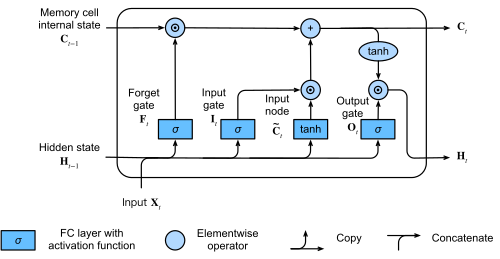
تحتوي الذاكرة طويلة المدى (LSTM) على آلية ذاكرة تعمل كوصلة متبقية. [ 4 ] في ذاكرة LSTM بدون بوابة نسيان ، يكون المدخلتتم معالجتها بواسطة دالةوأضيف إلى خلية ذاكرة، مما أدى إلى. تعمل شبكة LSTM المزودة ببوابة نسيان بشكل أساسي كشبكة طرق سريعة .


لتحقيق استقرار في تباين مدخلات الطبقات، يوصى باستبدال الوصلات المتبقيةمع، أينيمثل العدد الإجمالي للطبقات المتبقية. [ 5 ]


اتصال العرض
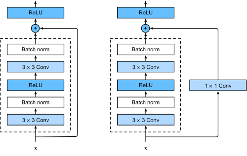
إذا كانت الدالةمن النوعأين، ثمغير مُعرَّف. لمعالجة هذه الحالة الخاصة، يتم استخدام اتصال إسقاطي:



أينعادةً ما يكون إسقاطًا خطيًا، يتم تحديده بواسطةأينهوالمصفوفة. يتم تدريب المصفوفة عبر الانتشار العكسي ، كما هو الحال مع أي معلمة أخرى للنموذج.


انتشار الإشارة
يُسهّل إدخال عمليات الربط المتطابقة انتشار الإشارة في كل من المسارات الأمامية والخلفية. [ 6 ]
الانتشار الأمامي
إذا كان ناتجالكتلة المتبقية رقم -th هي المدخل إلىالكتلة المتبقية رقم - (بافتراض عدم وجود دالة تنشيط بين الكتل)، ثمالمدخل رقم -th هو:


بتطبيق هذه الصيغة بشكل متكرر، على سبيل المثال:

ينتج عنه العلاقة العامة التالية:

أينهو فهرس كتلة متبقية ويمثل هذا فهرس كتلة سابقة. تشير هذه الصيغة إلى وجود إشارة تُرسل دائمًا مباشرةً من كتلة أقل عمقًا.إلى كتلة أعمق.


الانتشار العكسي
تُوفر صياغة التعلم المتبقي ميزة إضافية تتمثل في التخفيف من مشكلة تلاشي التدرج إلى حد ما. مع ذلك، من الضروري إدراك أن مشكلة تلاشي التدرج ليست السبب الجذري لمشكلة التدهور، والتي تُعالج باستخدام التطبيع. لملاحظة تأثير الكتل المتبقية على الانتشار العكسي، لننظر إلى المشتق الجزئي لدالة الخسارة .فيما يتعلق ببعض مدخلات الكتلة المتبقيةباستخدام المعادلة أعلاه من الانتشار الأمامي لكتلة متبقية لاحقة[ 6 ]


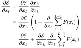
تشير هذه الصيغة إلى أن حساب التدرج لطبقة أقل عمقًا،، دائماً ما يكون له مصطلح لاحقتُضاف هذه القيمة مباشرةً. حتى لو كانت تدرجاتالحدود صغيرة، والتدرج الكلييقاوم التلاشي بسبب المصطلح المضاف.


أنواع مختلفة من الكتل المتبقية
الكتلة الأساسية
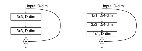
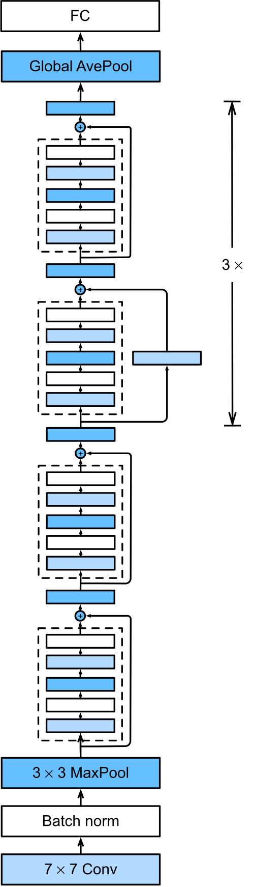
A basic block is the simplest building block studied in the original ResNet.[1] This block consists of two sequential 3x3 convolutional layers and a residual connection. The input and output dimensions of both layers are equal.
Bottleneck block
A bottleneck block[1] consists of three sequential convolutional layers and a residual connection. The first layer in this block is a 1×1 convolution for dimension reduction (e.g., to 1/2 of the input dimension); the second layer performs a 3×3 convolution; the last layer is another 1×1 convolution for dimension restoration. The models of ResNet-50, ResNet-101, and ResNet-152 are all based on bottleneck blocks.[1]
Pre-activation block
The pre-activation residual block[6] applies activation functions before applying the residual function . Formally, the computation of a pre-activation residual block can be written as:

where can be any activation (e.g. ReLU) or normalization (e.g. LayerNorm) operation. This design reduces the number of non-identity mappings between residual blocks, and allows an identity mapping directly from the input to the output. This design was used to train models with 200 to over 1000 layers, and was found to consistently outperform variants where the residual path is not an identity function. The pre-activation ResNet with 200 layers took 3 weeks to train for ImageNet on 8 GPUs in 2016.[6]

Since GPT-2, transformer blocks have been mostly implemented as pre-activation blocks. This is often referred to as "pre-normalization" in the literature of transformer models.[7]
Applications
Originally, ResNet was designed for computer vision.[1][8][9]
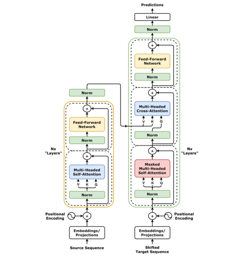
All transformer architectures include residual connections. Indeed, very deep transformers cannot be trained without them.[10]
The original ResNet paper made no claim on being inspired by biological systems. However, later research has related ResNet to biologically-plausible algorithms.[11][12]
A study published in Science in 2023[13] disclosed the complete connectome of an insect brain (specifically that of a fruit fly larva). This study discovered "multilayer shortcuts" that resemble the skip connections in artificial neural networks, including ResNets.
History
Previous work
Residual connections were noticed in neuroanatomy, such as Lorente de No (1938).[14]:Fig 3McCulloch and Pitts (1943) proposed artificial neural networks and considered those with residual connections.[15]:Fig 1.h
In 1961, Frank Rosenblatt described a three-layer multilayer perceptron (MLP) model with skip connections.[16]:313,Chapter 15 The model was referred to as a "cross-coupled system", and the skip connections were forms of cross-coupled connections.
During the late 1980s, "skip-layer" connections were sometimes used in neural networks. Examples include:[17][18] Lang and Witbrock (1988)[19] trained a fully connected feedforward network where each layer skip-connects to all subsequent layers, like the later DenseNet (2016). In this work, the residual connection was the form , where is a randomly-initialized projection connection. They termed it a "short-cut connection". An early neural language model used residual connections and named them "direct connections".[20]

Degradation problem
Sepp Hochreiter discovered the vanishing gradient problem in 1991[21] and argued that it explained why the then-prevalent forms of recurrent neural networks did not work for long sequences. He and Schmidhuber later designed the LSTM architecture to solve this problem,[4][22] which has a "cell state" that can function as a generalized residual connection. The highway network (2015)[23][24] applied the idea of an LSTM unfolded in time to feedforward neural networks, resulting in the highway network. ResNet is equivalent to an open-gated highway network.

During the early days of deep learning, there were attempts to train increasingly deep models. Notable examples included the AlexNet (2012), which had 8 layers, and the VGG-19 (2014), which had 19 layers.[25] However, stacking too many layers led to a steep reduction in training accuracy,[26] known as the "degradation" problem.[1] In theory, adding additional layers to deepen a network should not result in a higher training loss, but this is what happened with VGGNet.[1] If the extra layers can be set as identity mappings, however, then the deeper network would represent the same function as its shallower counterpart. There is some evidence that the optimizer is not able to approach identity mappings for the parameterized layers, and the benefit of residual connections was to allow identity mappings by default.[6]
In 2014, the state of the art was training deep neural networks with 20 to 30 layers.[25] The research team for ResNet attempted to train deeper ones by empirically testing various methods for training deeper networks, until they came upon the ResNet architecture.[27]
Subsequent work
Wide Residual Network (2016) found that using more channels and fewer layers than the original ResNet improves performance and GPU-computational efficiency, and that a block with two 3×3 convolutions is superior to other configurations of convolution blocks.[28]
DenseNet (2016)[29] connects the output of each layer to the input to each subsequent layer:

Stochastic depth[30] is a regularization method that randomly drops a subset of layers and lets the signal propagate through the identity skip connections. Also known as DropPath, this regularizes training for deep models, such as vision transformers.[31]
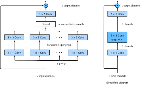
ResNeXt (2017) combines the Inception module with ResNet.[32][8]
Squeeze-and-Excitation Networks (2018) added squeeze-and-excitation (SE) modules to ResNet.[33] An SE module is applied after a convolution, and takes a tensor of shape (height, width, channels) as input. Each channel is averaged, resulting in a vector of shape . This is then passed through a multilayer perceptron (with an architecture such as linear-ReLU-linear-sigmoid) before it is multiplied with the original tensor. It won the ILSVRC in 2017.[34]


References
- 123456789He, Kaiming; Zhang, Xiangyu; Ren, Shaoqing; Sun, Jian (2016). Deep Residual Learning for Image Recognition(PDF). Conference on Computer Vision and Pattern Recognition. arXiv:1512.03385. doi:10.1109/CVPR.2016.90.
- ↑"ILSVRC2015 Results". image-net.org.
- ↑Deng, Jia; Dong, Wei; Socher, Richard; Li, Li-Jia; Li, Kai; Li, Fei-Fei (2009). ImageNet: A large-scale hierarchical image database. Conference on Computer Vision and Pattern Recognition. doi:10.1109/CVPR.2009.5206848.
- 12Sepp Hochreiter; Jürgen Schmidhuber (1997). "Long short-term memory". Neural Computation. 9 (8): 1735–1780. doi:10.1162/neco.1997.9.8.1735. PMID 9377276. S2CID 1915014.
- ↑Hanin, Boris; Rolnick, David (2018). How to Start Training: The Effect of Initialization and Architecture(PDF). Conference on Neural Information Processing Systems. Vol. 31. Curran Associates, Inc. arXiv:1803.01719.
- 1 2 3 4 5 هو, كايمينغ ; تشانغ، شيانغيو. رن، شاوتشينج؛ صن ، جيان (2016). تعيينات الهوية في الشبكات العميقة المتبقية (PDF) . المؤتمر الأوروبي حول رؤية الكمبيوتر . أرخايف : 1603.05027 . دوى : 10.1007/978-3-319-46493-0_38 .
- ↑ رادفورد، أليك؛ وو، جيفري؛ تشايلد، ريون؛ لوان، ديفيد؛ أمودي، داريو؛ سوتسكيفر، إيليا (14 فبراير 2019). "نماذج اللغة هي متعلمون متعددون المهام غير خاضعين للإشراف" (ملف PDF) . مؤرشف (PDF) من الأصل في 6 فبراير 2021. تم الاطلاع عليه في 19 ديسمبر 2020 .
- 1 2 3 تشانغ، أستون؛ ليبتون، زاكاري؛ لي، مو؛ سمولا، ألكسندر ج. (2024). "8.6. الشبكات المتبقية (ResNet) وResNeXt" . تعمق في التعلم العميق . كامبريدج، نيويورك، بورت ملبورن، نيودلهي، سنغافورة: مطبعة جامعة كامبريدج. ISBN 978-1-009-38943-3.
- ↑ سيجيدي، كريستيان؛ إيوف، سيرجي؛ فان هوك، فينسنت؛ أليمي، أليكس (2017). Inception-v4، Inception-ResNet وتأثير الاتصالات المتبقية على التعلم (ملف PDF) . مؤتمر AAAI حول الذكاء الاصطناعي . arXiv : 1602.07261 . doi : 10.1609/aaai.v31i1.11231 .
- ↑ دونغ، ييهي؛ كوردونييه، جان بابتيست؛ لوكاس، أندرياس (2021). الانتباه ليس كل ما تحتاجه: الانتباه الخالص يفقد رتبته بشكل مضاعف أُسّيًا مع العمق (ملف PDF) . المؤتمر الدولي للتعلم الآلي . PMLR. الصفحات 2793-2803 . arXiv : 2103.03404 .
- ↑ لياو، تشيانلي؛ بوجيو، توماسو (2016). "سد الفجوات بين التعلم المتبقي، والشبكات العصبية المتكررة، والقشرة البصرية". arXiv : 1604.03640 [ cs.LG ].
- ↑ شياو، ويل؛ تشين، هونغلين؛ لياو، تشيانلي؛ بوجيو، توماسو (2019). خوارزميات التعلم ذات المعقولية البيولوجية قابلة للتوسع لتشمل مجموعات البيانات الكبيرة . المؤتمر الدولي حول تمثيلات التعلم . arXiv : 1811.03567 .
- ↑ ويندينغ، مايكل؛ بيديجو، بنجامين؛ بارنز، كريستوفر؛ باتسوليك، هيذر؛ بارك، يونغسر؛ كازيميرز، توم؛ فوشيكي، أكيرا؛ أندرادي، إنغريد؛ خانديلوال، أفيناش؛ فالديس-أليمان، خافيير؛ لي، فينغ؛ راندل، نادين؛ بارسوتي، إليزابيث؛ كوريا، آنا؛ فيتر، فيتر؛ هارتنشتاين، فولكر؛ بريبي، كاري؛ فوغلشتاين، جوشوا؛ كاردونا، ألبرت ؛ زلاتيتش، مارتا (10 مارس 2023). "الشبكة العصبية لدماغ حشرة" . مجلة ساينس . 379 (6636) eadd9330. bioRxiv 10.1101/2022.11.28.516756v1 . doi : 10.1126/science.add9330 . PMC 7614541 . PMID 36893230 . S2CID 254070919 .
- ↑ دي ن، رافائيل لورينتي (1938-05-01). "تحليل نشاط سلاسل الخلايا العصبية البينية" . مجلة علم وظائف الأعصاب . 1 (3): 207-244 . doi : 10.1152/jn.1938.1.3.207 . ISSN 0022-3077 .
- ↑ ماكولوتش، وارن س.؛ بيتس، والتر (1943-12-01). "حساب منطقي للأفكار الكامنة في النشاط العصبي" . نشرة الفيزياء الحيوية الرياضية . 5 (4): 115-133 . doi : 10.1007/BF02478259 . ISSN 1522-9602 .
- ↑ روزنبلات، فرانك (1961). مبادئ الديناميكا العصبية. البيرسيبترونات ونظرية آليات الدماغ (PDF) .
- ↑ روميلهارت، ديفيد إي، وجيفري إي. هينتون، ورونالد جيه. ويليامز. "تعلم التمثيلات الداخلية عن طريق نشر الخطأ"، المعالجة الموزعة المتوازية . المجلد 1. 1986.
- ↑ فينابلز، دبليو إن؛ ريبلي، براين دي. (1994). الإحصاء التطبيقي الحديث باستخدام إس-بلس . سبرينغر. ص 261-262 . ISBN 978-3-540-94350-1.
- ↑ لانغ، كيفن؛ ويتبروك، مايكل (1988). "تعلم التمييز بين حلزونين" (ملف PDF) . وقائع المدرسة الصيفية لنماذج الاتصال لعام 1988 : 52-59 .
- ↑ بينجيو، يوشوا ؛ دوشارم، ريجان؛ فنسنت، باسكال؛ جوفان، كريستيان (2003). "نموذج لغوي احتمالي عصبي" . مجلة أبحاث تعلم الآلة . 3 (فبراير): 1137-1155 . ISSN 1533-7928 .
- ^ هوخريتر، سيب (1991). Unter suchungen zu dynamischen neuronalen Netzen (PDF) (أطروحة الدبلوم). جامعة ميونيخ التقنية ، معهد علوم الكمبيوتر، المستشار: ج. شميدهوبر.
- ↑ فيليكس أ. جيرز؛ يورغن شميدهوبر؛ فريد كامينز (2000). " التعلم من النسيان: التنبؤ المستمر باستخدام LSTM". الحوسبة العصبية . 12 (10): 2451-2471 . CiteSeerX 10.1.1.55.5709 . doi : 10.1162/089976600300015015 . PMID 11032042. S2CID 11598600 .
- ^ سريفاستافا، روبيش كومار؛ جريف، كلاوس. شميدهوبر، يورغن (3 مايو 2015). “شبكات الطرق السريعة”. أرخايف : 1505.00387 [ cs.LG ].
- ↑ سريفاستافا، روبيش كومار؛ جريف، كلاوس؛ شميدهوبر، يورغن (2015). تدريب الشبكات العميقة جدًا (ملف PDF) . مؤتمر أنظمة معالجة المعلومات العصبية . arXiv : 1507.06228 .
- 1 2 سيمونيان، كارين؛ زيسرمان، أندرو (2015-04-10). "شبكات الالتفاف العميقة جدًا للتعرف على الصور واسعة النطاق". arXiv : 1409.1556 [ cs.CV ].
- ↑ هي، كايمينغ ؛ تشانغ، شيانغيو؛ رين، شاوكينغ؛ صن، جيان (2015). التعمق في المُقوِّمات: تجاوز مستوى الأداء البشري في تصنيف ImageNet (ملف PDF) . المؤتمر الدولي لرؤية الحاسوب . arXiv : 1502.01852 . doi : 10.1109/ICCV.2015.123 .
- ↑ لين، أليسون (10 ديسمبر 2015). "باحثو مايكروسوفت يفوزون بتحدي ImageNet للرؤية الحاسوبية" . مدونة الذكاء الاصطناعي . مؤرشف من الأصل بتاريخ 29 يناير 2018. تم الاطلاع عليه بتاريخ 29 يونيو 2024 .
- ↑ زاغورويكو، سيرجي؛ كوموداكيس، نيكوس (2016-05-23). "الشبكات المتبقية الواسعة". arXiv : 1605.07146 [ cs.CV ].
- ↑ هوانغ، غاو؛ ليو، تشوانغ؛ فان دير ماتن، لورينز؛ واينبرغر، كيليان (2017). الشبكات الالتفافية المتصلة بكثافة (ملف PDF) . مؤتمر رؤية الحاسوب والتعرف على الأنماط . arXiv : 1608.06993 . doi : 10.1109/CVPR.2017.243 .
- ↑ هوانغ، غاو؛ صن، يو؛ ليو، تشوانغ؛ واينبرغر، كيليان (2016). الشبكات العميقة ذات العمق العشوائي (ملف PDF) . المؤتمر الأوروبي لرؤية الحاسوب . arXiv : 1603.09382 . doi : 10.1007/978-3-319-46493-0_39 .
- ↑ لي، يونغوان؛ كيم، جونغهي؛ ويلت، جيفري؛ هوانغ، سونغ جو (2022). MPViT: مُحوِّل الرؤية متعدد المسارات للتنبؤ الكثيف (ملف PDF) . مؤتمر رؤية الحاسوب والتعرف على الأنماط . الصفحات 7287-7296 . arXiv : 2112.11010 . doi : 10.1109/CVPR52688.2022.00714 .
- ↑ شي، ساينينغ؛ غيرشيك، روس؛ دولار، بيوتر؛ تو، تشووين؛ هي، كايمينغ (2017). تحويلات البقايا المجمعة للشبكات العصبية العميقة (ملف PDF) . مؤتمر رؤية الحاسوب والتعرف على الأنماط . الصفحات 1492-1500 . arXiv : 1611.05431 . doi : 10.1109/CVPR.2017.634 .
- ↑ هو، جي؛ شين، لي؛ صن، غانغ (2018). شبكات الضغط والإثارة (ملف PDF) . مؤتمر رؤية الحاسوب والتعرف على الأنماط . الصفحات 7132-7141 . arXiv : 1709.01507 . doi : 10.1109/CVPR.2018.00745 .
- ↑ جي، هو (2017). شبكات الضغط والإثارة (ملف PDF) . ما وراء تحدي التعرف البصري واسع النطاق ImageNet، ورشة عمل في مؤتمر CVPR 2017 (عرض تقديمي).
- بنى الشبكات العصبية
- التعلم العميق