
Musical isomorphism
In mathematics—more specifically, in differential geometry—the musical isomorphism (or canonical isomorphism) is an isomorphism between the tangent bundle and the cotangent bundle of a Riemannian or pseudo-Riemannian manifold induced by its metric tensor. There are similar isomorphisms on symplectic manifolds. These isomorphisms are global versions of the canonical isomorphism between an inner product space and its dual. The term musical refers to the use of the musical notation symbols (flat) and (sharp).[1][2]


In the notation of Ricci calculus and mathematical physics, the idea is expressed as the raising and lowering of indices. Raising and lowering indices are a form of index manipulation in tensor expressions.
In certain specialized applications, such as on Poisson manifolds, the relationship may fail to be an isomorphism at singular points, and so, for these cases, is technically only a homomorphism.
Motivation
The index-raising isomorphism is a coordinate-free way to define the gradient of a function from its exterior derivative.

In linear algebra, a finite-dimensional vector space is isomorphic to its dual space (the space of linear functionals mapping the vector space to its base field), but not canonically. Given a fixed basis for this vector space, there is a natural way to go back and forth between vectors and linear forms: vectors are represented in the basis by column vectors, linear forms are represented in the basis by row vectors, and the identification is done by transposition.
On the other hand, a finite-dimensional vector space endowed with a non-degenerate bilinear form is canonically isomorphic to its dual. The canonical isomorphism is given by


- .

An example is where and is the dot product.

In a basis , the canonical isomorphism above can be described as follows. Let be the components of the non-degenerate bilinear form and let be the components of the inverse matrix to . Let be the dual basis of . A vector is written in the basis as using Einstein summation notation, i.e., has components in the basis. The canonical isomorphism applied to gives an element of the dual, which is called a covector. The covector has components in the dual basis given by contracting with :


This is what is meant by lowering the index. Conversely, contracting a covector with the inverse of gives a vector with components


in the basis . This process is called raising the index.
Raising and then lowering the same index (or conversely) are inverse operations, which is reflected in and being inverses:

where is the Kronecker delta or identity matrix.

The musical isomorphisms are the global version of the canonical isomorphism and its inverse for the tangent bundle and cotangent bundle of a (pseudo-)Riemannian manifold . They are canonical isomorphisms of vector bundles that are defined on every tangent space for by and its inverse


Because every smooth manifold can be (non-canonically) endowed with a Riemannian metric, the musical isomorphisms show that a vector bundle on a smooth manifold is (non-canonically) isomorphic to its dual.
Abstractly, the musical isomorphisms can be understood as a currying of the bilinear form.
Discussion
Let be a (pseudo-)Riemannian manifold. At each point , the map is a non-degenerate bilinear form on the tangent space . If is a vector in , its flat is the covector


in . Since this is a smooth map that preserves the point , it defines a morphism of smooth vector bundles :\mathrm {T} M\to \mathrm {T} ^{*}M} . By non-degeneracy of the metric, has an inverse at each point, characterized by


for in and in . The vector is called the sharp of . The sharp map is a smooth bundle map :\mathrm {T} ^{*}M\to \mathrm {T} M} .


Flat and sharp are mutually inverse isomorphisms of smooth vector bundles, hence, for each in , there are mutually inverse vector space isomorphisms between and .

The flat and sharp maps can be applied to vector fields and covector fields by applying them to each point. Hence, if is a vector field and is a covector field,


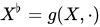
and
- .

In a moving frame
Suppose {ei} is a moving tangent frame (see also smooth frame) for the tangent bundle TM with, as dual frame (see also dual basis), the moving coframe (a moving tangent frame for the cotangent bundle; see also coframe) {ei}. Then the pseudo-Riemannian metric, which is a 2-covariant tensor field, can be written locally in this coframe as g = gijei ⊗ ej using Einstein summation notation.
Given a vector field X = Xiei and denoting gijXi = Xj, its flat is
- .

This is referred to as lowering an index, because the components of X are written with an upper index Xi, whereas the components of are written with a lower index Xj.

In the same way, given a covector field ω = ωiei and denoting gijωi = ωj, its sharp is
- ,

where gij are the components of the inverse metric tensor (given by the entries of the inverse matrix to gij). Taking the sharp of a covector field is referred to as raising an index.
Extension to tensor products
The musical isomorphisms may also be extended, for each r, s, k, to an isomorphism between the bundle

of tensors and the bundle of tensors. Here k can be positive or negative, so long as r - k ≥ 0 and s + k ≥ 0.


Lowering an index of an tensor gives a tensor, while raising an index gives a . Which index is to be raised or lowered must be indicated.
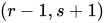
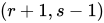
For instance, consider the (0, 2) tensor X = Xijei ⊗ ej. Raising the second index, we get the (1, 1) tensor

In other words, the components of are given by


Similar formulas are available for tensors of other orders. For example, for a tensor X, all indices are raised by:[3]


For a tensor X, all indices are lowered by:


For a mixed tensor of order , all lower indices are raised and all upper indices are lowered by


Well-formulated expressions are constrained by the rules of Einstein summation notation: any index may appear at most twice and furthermore a raised index must contract with a lowered index. With these rules we can immediately see that an expression such as is well formulated while is not.


Extension to k-vectors and k-forms
In the context of exterior algebra, an extension of the musical operators may be defined on ⋀V and its dual ⋀V*, and are again mutual inverses:[4]
- :\bigwedge _{i=1}^{k}V\to \bigwedge _{i=1}^{k}V^{*},}
- :\bigwedge _{i=1}^{k}V^{*}\to \bigwedge _{i=1}^{k}V,}


defined by


In this extension, in which ♭ maps k-vectors to k-covectors and ♯ maps k-covectors to k-vectors, all the indices of a totally antisymmetric tensor are simultaneously raised or lowered, and so no index need be indicated:

This works not just for k-vectors in the context of linear algebra but also for k-forms in the context of a (pseudo-)Riemannian manifold:
- :\bigwedge _{i=1}^{k}{\rm {T}}M\to \bigwedge _{i=1}^{k}{\rm {T}}^{*}M,}
- :\bigwedge _{i=1}^{k}{\rm {T}}^{*}M\to \bigwedge _{i=1}^{k}{\rm {T}}M,}


Vector bundles with bundle metrics
More generally, musical isomorphisms always exist between a vector bundle endowed with a bundle metric and its dual.
Trace of a tensor
Given a (0, 2) tensor X = Xijei ⊗ ej, we define the trace of X through the metric tensor g by

Observe that the definition of trace is independent of the choice of index to raise, since the metric tensor is symmetric.
The trace of an tensor can be taken in a similar way, so long as one specifies which two distinct indices are to be traced. This process is also called contracting the two indices. For example, if X is an tensor with r > 1, then the indices and can be contracted to give an tensor with components


Example computations
In Minkowski spacetime
The covariant 4-position is given by

with components:

(where x,y,z are the usual Cartesian coordinates) and the Minkowski metric tensor with metric signature (− + + +) is defined as
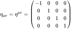
in components:

To raise the index, multiply by the tensor and contract:

then for λ = 0:

and for λ = j = 1, 2, 3:

So the index-raised contravariant 4-position is:

This operation is equivalent to the matrix multiplication

Given two vectors, and , we can write down their (pseudo-)inner product in two ways:


By lowering indices, we can write this expression as

In matrix notation, the first expression can be written as
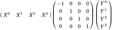
while the second is, after lowering the indices of ,
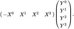
In electromagnetism
For a (0,2) tensor,[3] twice contracting with the inverse metric tensor and contracting in different indices raises each index:

Similarly, twice contracting with the metric tensor and contracting in different indices lowers each index:

Let's apply this to the theory of electromagnetism.
The contravariantelectromagnetic tensor in the (+ − − −)signature is given by[5]
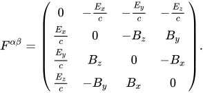
In components,

To obtain the covariant tensor Fαβ, contract with the inverse metric tensor:

and since F00 = 0 and F0i = − Fi0, this reduces to

Now for α = 0, β = k = 1, 2, 3:
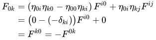
and by antisymmetry, for α = k = 1, 2, 3, β = 0:

then finally for α = k = 1, 2, 3, β = l = 1, 2, 3;
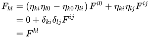
The (covariant) lower indexed tensor is then:
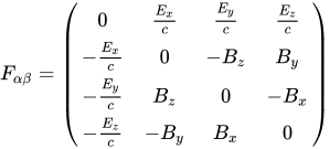
This operation is equivalent to the matrix multiplication

See also
Citations
- ↑Lee 2003, Chapter 11.
- ↑Lee 1997, Chapter 3.
- 12Kay, D. C. (1988). Tensor Calculus. Schaum’s Outlines. New York: McGraw Hill. ISBN 0-07-033484-6.
- ↑Vaz & da Rocha 2016, pp. 48, 50.
- ↑NB: Some texts, such as: Griffiths, David J. (1987). Introduction to Elementary Particles. Wiley, John & Sons, Inc. ISBN 0-471-60386-4., will show this tensor with an overall factor of −1. This is because they used the negative of the metric tensor used here: (− + + +), see metric signature. In older texts such as Jackson (2nd edition), there are no factors of c since they are using Gaussian units. Here SI units are used.
References
- Lee, J. M. (2003). Introduction to Smooth manifolds. Springer Graduate Texts in Mathematics. Vol. 218. ISBN 0-387-95448-1.
- Lee, J. M. (1997). Riemannian Manifolds – An Introduction to Curvature. Springer Graduate Texts in Mathematics. Vol. 176. Springer Verlag. ISBN 978-0-387-98322-6.
- Vaz, Jayme; da Rocha, Roldão (2016). An Introduction to Clifford Algebras and Spinors. Oxford University Press. ISBN 978-0-19-878-292-6.
- Differential geometry
- Riemannian geometry
- Riemannian manifolds
- Symplectic geometry