مرشح خطي

تقوم المرشحات الخطية بمعالجة إشارات الدخل المتغيرة مع الزمن لإنتاج إشارات خرج، مع مراعاة شرط الخطية . في معظم الحالات، تكون هذه المرشحات الخطية ثابتة مع الزمن (أو ثابتة مع الإزاحة )، وفي هذه الحالة يمكن تحليلها بدقة باستخدام نظرية الأنظمة الخطية الثابتة مع الزمن (LTI)، مما يكشف عن دوال نقلها في مجال التردد واستجاباتها النبضية في مجال الزمن. تُعدّ التطبيقات الآنية لمثل هذه المرشحات الخطية لمعالجة الإشارات في مجال الزمن سببية حتمًا ، وهو قيد إضافي على دوال نقلها. تندرج الدوائر الإلكترونية التناظرية التي تتكون فقط من مكونات خطية (مقاومات، مكثفات، ملفات حث، ومضخمات خطية) بالضرورة ضمن هذه الفئة، وكذلك الأنظمة الميكانيكية المماثلة أو أنظمة معالجة الإشارات الرقمية التي تحتوي على عناصر خطية فقط. ونظرًا لإمكانية توصيف المرشحات الخطية الثابتة مع الزمن بشكل كامل من خلال استجابتها لموجات جيبية ذات ترددات مختلفة ( استجابة التردد )، فإنها تُعرف أحيانًا باسم مرشحات التردد.

لا يشترط أن تكون تطبيقات المرشحات الخطية الثابتة زمنيًا غير الآنية سببية. كما تُستخدم مرشحات متعددة الأبعاد، كما هو الحال في معالجة الصور . ويمتد المفهوم العام للتصفية الخطية إلى مجالات وتقنيات أخرى، مثل الإحصاء وتحليل البيانات والهندسة الميكانيكية .

استجابة النبضة ووظيفة النقل

يمكن تحديد مرشح خطي ثابت مع الزمن (LTI) بشكل فريد من خلال استجابته النبضية h ، ويُعبّر رياضيًا عن خرج أي مرشح على أنه التفاف المدخل مع تلك الاستجابة النبضية. أما الاستجابة الترددية ، فتُعطى بواسطة دالة نقل المرشح. $H(\omega )$ يُعدّ هذا وصفًا بديلًا للمرشح. تتمثل الأهداف النموذجية لتصميم المرشحات في تحقيق استجابة ترددية معينة، أي مقدار دالة النقل. $|H(\omega )|$ تختلف أهمية طور دالة النقل باختلاف التطبيق، إذ يمكن تشويه شكل الموجة بدرجة أو بأخرى أثناء عملية تحقيق استجابة (سعة) مطلوبة في مجال التردد. ويمكن تعديل استجابة التردد، على سبيل المثال، لإزالة مكونات التردد غير المرغوب فيها من إشارة الدخل ، أو لحصر عمل المضخم على الإشارات ضمن نطاق ترددي محدد.

The impulse responseh of a linear time-invariant causal filter specifies the output that the filter would produce if it were to receive an input consisting of a single impulse at time 0. An "impulse" in a continuous time filter means a Dirac delta function; in a discrete time filter the Kronecker delta function would apply. The impulse response completely characterizes the response of any such filter, inasmuch as any possible input signal can be expressed as a (possibly infinite) combination of weighted delta functions. Multiplying the impulse response shifted in time according to the arrival of each of these delta functions by the amplitude of each delta function, and summing these responses together (according to the superposition principle, applicable to all linear systems) yields the output waveform.

Mathematically this is described as the convolution of a time-varying input signal x(t) with the filter's impulse responseh, defined as:

y(t)=\int _{0}^{T}x(t-\tau )\,h(\tau )\,d\tau

or

y_{k}=\sum _{i=0}^{N}x_{k-i}\,h_{i}

.

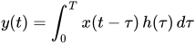
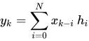
The first form is the continuous-time form, which describes mechanical and analog electronic systems, for instance. The second equation is a discrete-time version used, for example, by digital filters implemented in software, so-called digital signal processing. The impulse response h completely characterizes any linear time-invariant (or shift-invariant in the discrete-time case) filter. The input x is said to be "convolved" with the impulse response h having a (possibly infinite) duration of time T (or of Nsampling periods).

Filter design consists of finding a possible transfer function that can be implemented within certain practical constraints dictated by the technology or desired complexity of the system, followed by a practical design that realizes that transfer function using the chosen technology. The complexity of a filter may be specified according to the order of the filter.

Among the time-domain filters we here consider, there are two general classes of filter transfer functions that can approximate a desired frequency response. Very different mathematical treatments apply to the design of filters termed infinite impulse response (IIR) filters, characteristic of mechanical and analog electronics systems, and finite impulse response (FIR) filters, which can be implemented by discrete time systems such as computers (then termed digital signal processing).

Implementation issues

Classical analog filters are IIR filters, and classical filter theory centers on the determination of transfer functions given by low order rational functions, which can be synthesized using the same small number of reactive components.^[1] Using digital computers, on the other hand, both FIR and IIR filters are straightforward to implement in software.

A digital IIR filter can generally approximate a desired filter response using less computing power than a FIR filter, however this advantage is more often unneeded given the increasing power of digital processors. The ease of designing and characterizing FIR filters makes them preferable to the filter designer (programmer) when ample computing power is available. Another advantage of FIR filters is that their impulse response can be made symmetric, which implies a response in the frequency domain that has zero phase at all frequencies (not considering a finite delay), which is absolutely impossible with any IIR filter.^[2]

Frequency response

The frequency response or transfer function $|H(\omega )|$ of a filter can be obtained if the impulse response is known, or directly through analysis using Laplace transforms, or in discrete-time systems the Z-transform. The frequency response also includes the phase as a function of frequency, however in many cases the phase response is of little or no interest. FIR filters can be made to have zero phase, but with IIR filters that is generally impossible. With most IIR transfer functions there are related transfer functions having a frequency response with the same magnitude but a different phase; in most cases the so-called minimum phase transfer function is preferred.

Filters in the time domain are most often requested to follow a specified frequency response. Then, a mathematical procedure finds a filter transfer function that can be realized (within some constraints), and approximates the desired response to within some criterion. Common filter response specifications are described as follows:

A low-pass filter passes low frequencies while blocking higher frequencies.
A high-pass filter passes high frequencies.
A band-pass filter passes a band (range) of frequencies.
A band-stop filter passes high and low frequencies outside of a specified band.
A notch filter has a null response at a particular frequency. This function may be combined with one of the above responses.
An all-pass filter passes all frequencies equally well, but alters the group delay and phase relationship among them.
An equalization filter is not designed to fully pass or block any frequency, but instead to gradually vary the amplitude response as a function of frequency: filters used as pre-emphasis filters, equalizers, or tone controls are good examples.

FIR transfer functions

Meeting a frequency response requirement with an FIR filter uses relatively straightforward procedures. In the most basic form, the desired frequency response itself can be sampled with a resolution of $\Delta f$ and Fourier transformed to the time domain. This obtains the filter coefficients h_i, which implements a zero phase FIR filter that matches the frequency response at the sampled frequencies used. To better match a desired response, $\Delta f$ must be reduced. However the duration of the filter's impulse response, and the number of terms that must be summed for each output value (according to the above discrete time convolution) is given by $N=1/(\Delta f\,T)$ where T is the sampling period of the discrete time system (N-1 is also termed the order of an FIR filter). Thus the complexity of a digital filter and the computing time involved, grows inversely with $\Delta f$ , placing a higher cost on filter functions that better approximate the desired behavior. For the same reason, filter functions whose critical response is at lower frequencies (compared to the sampling frequency1/T) require a higher order, more computationally intensive FIR filter. An IIR filter can thus be much more efficient in such cases.

Elsewhere the reader may find further discussion of design methods for practical FIR filter design.

IIR transfer functions

بما أن المرشحات التناظرية الكلاسيكية هي مرشحات IIR، فقد كان هناك تاريخ طويل من دراسة نطاق دوال النقل الممكنة التي تُنفذ استجابات المرشح المطلوبة في أنظمة الزمن المستمر. باستخدام التحويلات، يُمكن تحويل استجابات التردد هذه في الزمن المستمر إلى استجابات تُنفذ في الزمن المتقطع، لاستخدامها في مرشحات IIR الرقمية. يُحدد تعقيد أي مرشح من هذا النوع بالرتبة N ، التي تصف رتبة الدالة الكسرية التي تصف استجابة التردد. تُعد الرتبة N ذات أهمية خاصة في المرشحات التناظرية، لأن المرشح الإلكتروني ^من الرتبة N يتطلب N عنصرًا تفاعليًا (مكثفات و/أو محاثات) لتنفيذه. إذا تم تنفيذ مرشح باستخدام، على سبيل المثال، مراحل ثنائية التربيع باستخدام مضخمات العمليات ، فستكون هناك حاجة إلى N/2 مرحلة. في التنفيذ الرقمي، يتناسب عدد العمليات الحسابية التي تُجرى لكل عينة مع N. وبالتالي، فإن المشكلة الرياضية هي الحصول على أفضل تقريب (بمعنى ما) للاستجابة المطلوبة باستخدام قيمة N أصغر، كما سنوضح الآن.

فيما يلي استجابات التردد لعدة دوال ترشيح قياسية تُقارب الاستجابة المطلوبة، مُحسَّنة وفقًا لمعيار مُحدد. جميعها مرشحات تمرير منخفض من الرتبة الخامسة، مُصممة لتردد قطع يبلغ 0.5 بوحدات مُعيَّرة. تُعرض استجابات التردد لمرشحات باترورث ، تشيبيشيف ، تشيبيشيف العكسي ، والمرشح الإهليلجي .

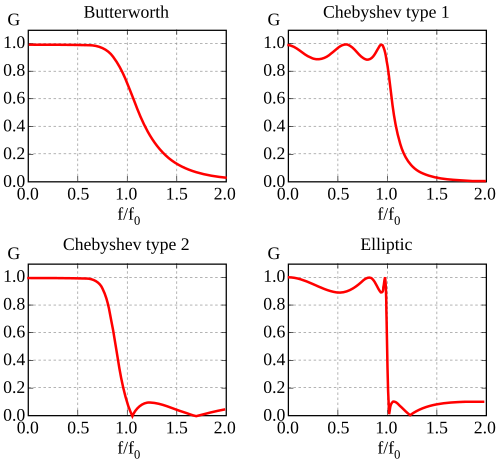
كما هو واضح من الصورة، يتميز المرشح الإهليلجي بحدة أعلى من غيره، لكن على حساب ظهور تموجات في نطاقي التمرير والإيقاف. أما مرشح باترورث، فيتميز بأضعف انتقال، ولكنه يوفر استجابة أكثر انتظامًا، متجنبًا التموجات في نطاقي التمرير والإيقاف. بينما يتميز مرشح بيسل (غير الموضح) بانتقال أضعف في مجال التردد، ولكنه يحافظ على أفضل دقة طور للموجة. وتتطلب التطبيقات المختلفة متطلبات تصميم مختلفة، مما يؤدي إلى خيارات متباينة بين هذه التحسينات (وغيرها)، أو قد يستلزم استخدام مرشح من رتبة أعلى.

أمثلة على التطبيقات

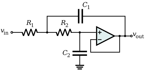
تُعدّ دائرة سالين-كي من الدوائر الشائعة التي تُنفّذ مرشح RC نشط من الدرجة الثانية، ويظهر مخططها هنا. ويمكن تكييف هذه الدائرة لإنتاج مرشحات تمرير منخفض، ومرشحات تمرير نطاقي، ومرشحات تمرير عالي.

^{يمكن تنفيذ مرشح FIR من الرتبة} N في نظام زمني منفصل باستخدام برنامج حاسوبي أو أجهزة متخصصة، حيث تخضع إشارة الدخل لـ N مرحلة تأخير. يتكون خرج المرشح من مجموع مرجح لهذه الإشارات المتأخرة، كما هو موضح في مخطط تدفق الإشارة المرفق. تعتمد استجابة المرشح على معاملات الترجيح b₀ _، b₁ _، ... ، bₙ _. على سبيل المثال، إذا كانت جميع المعاملات تساوي واحدًا، وهو ما يُعرف بدالة الصندوق ، فسيتم تنفيذ مرشح تمرير منخفض بكسب تردد منخفض N+1 واستجابة ترددية معطاة بدالة sinc . يمكن الحصول على أشكال أفضل للاستجابة الترددية باستخدام معاملات مشتقة من إجراء تصميم أكثر تطورًا.

رياضيات تصميم المرشحات

تصف نظرية الأنظمة الخطية الثابتة مع الزمن (LTI) جميع أنواع المرشحات الخطية الثابتة مع الزمن. يمكن وصف مرشحات LTI وصفًا كاملًا من خلال استجابتها الترددية واستجابتها الطورية ، حيث يحدد تحديد هاتين الاستجابتين استجابتها النبضية بشكل فريد ، والعكس صحيح . من وجهة نظر رياضية، يمكن وصف مرشحات LTI ذات الاستجابة النبضية اللانهائية (IIR) المستمرة باستخدام المعادلات التفاضلية الخطية ، مع اعتبار استجاباتها النبضية دوال غرين لهذه المعادلات. كما يمكن وصف مرشحات LTI المستمرة باستخدام تحويل لابلاس لاستجابتها النبضية، مما يسمح بتحليل جميع خصائص المرشح من خلال دراسة نمط أصفار وأقطاب تحويل لابلاس في المستوى المركب . وبالمثل، يمكن تحليل مرشحات LTI المتقطعة باستخدام تحويل Z لاستجابتها النبضية.

قبل ظهور أدوات توليف المرشحات الحاسوبية، كانت الأدوات الرسومية، مثل مخططات بود ومخططات نايكويست، تُستخدم على نطاق واسع كأدوات تصميم. وحتى اليوم، لا تزال هذه الأدوات بالغة الأهمية لفهم سلوك المرشحات. احتوت المراجع ^{[ 3 ]} على رسومات بيانية شاملة لاستجابة التردد، واستجابة الطور، وتأخير المجموعة، واستجابة النبضة لأنواع مختلفة من المرشحات، وبمختلف الرتب. كما احتوت على جداول قيم توضح كيفية تنفيذ هذه المرشحات على شكل سلالم RLC، وهو أمر مفيد للغاية عندما كانت عناصر التضخيم باهظة الثمن مقارنةً بالمكونات السلبية. ويمكن أيضًا تصميم مثل هذا السلم بحيث يكون ذا حساسية ضئيلة لتغيرات المكونات، وهي خاصية يصعب تقييمها بدون أدوات حاسوبية.

Many different analog filter designs have been developed, each trying to optimise some feature of the system response. For practical filters, a custom design is sometimes desirable, that can offer the best tradeoff between different design criteria, which may include component count and cost, as well as filter response characteristics.

These descriptions refer to the mathematical properties of the filter (that is, the frequency and phase response). These can be implemented as analog circuits (for instance, using a Sallen Key filter topology, a type of active filter), or as algorithms in digital signal processing systems.

Digital filters are much more flexible to synthesize and use than analog filters, where the constraints of the design permits their use. Notably, there is no need to consider component tolerances, and very high Q levels may be obtained.

FIR digital filters may be implemented by the direct convolution of the desired impulse response with the input signal. They can easily be designed to give a matched filter for any arbitrary pulse shape.

IIR digital filters are often more difficult to design, due to problems including dynamic range issues, quantization noise and instability. Typically digital IIR filters are designed as a series of digital biquad filters.

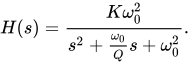
All low-pass second-order continuous-time filters have a transfer function given by

H(s)={\frac {K\omega _{0}^{2}}{s^{2}+{\frac {\omega _{0}}{Q}}s+\omega _{0}^{2}}}.

All band-pass second-order continuous-time filters have a transfer function given by

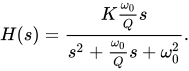
H(s)={\frac {K{\frac {\omega _{0}}{Q}}s}{s^{2}+{\frac {\omega _{0}}{Q}}s+\omega _{0}^{2}}}.

where

K is the gain (low-pass DC gain, or band-pass mid-band gain) (K is 1 for passive filters)
Q is the Q factor
$\omega _{0}$ is the center frequency
$s=\sigma +j\omega$ is the complex frequency

Notes and references

↑However, there are a few cases in which FIR filters directly process analog signals, involving non-feedback topologies and analog delay elements. An example is the discrete-time analog sampled filter, implemented using a so-called bucket-brigade device clocked at a certain sampling rate, outputting copies of the input signal at different delays that can be combined with some weighting to realize an FIR filter. Electromechanical filters such as SAW filters can likewise implement FIR filter responses; these operate in continuous time and can thus be designed for higher frequencies.
↑Outside of trivial cases, stable IIR filters with zero phase response are possible if they are not causal (and thus are unusable in real-time applications) or implementing transfer functions classified as unstable or "marginally stable" such as a double integrator.
↑A. Zverev, Handbook of Filter Synthesis, John Wiley and Sons, 1967, ISBN 0-471-98680-1

اللغة	العربية (RTL)
روابط موسوعية	30 رابطاً
المصدر الأصلي	ويكيبيديا ↗