Periodic table of topological insulators and topological superconductors

The non-chiral Su–Schrieffer–Heeger model (${\displaystyle d=1}$), can be associated with symmetry class BDI with an integer ${\displaystyle \mathbb {Z} }$ topological invariant due to gauge invariance.^[6][7] The problem is similar to the integer quantum Hall effect and the quantum anomalous Hall effect (both in ${\displaystyle d=2}$) which are A class, with integer ${\displaystyle \mathbb {Z} }$Chern number.^[8]

Contrarily, the Kitaev chain (${\displaystyle d=1}$) is also in BDI class, but in the presence of a magnetic field it becomes an example of symmetry class D, with a ${\displaystyle \mathbb {Z} _{2}}$ binary topological invariant.^[7] Similarly, the ${\displaystyle p_{x}+ip_{y}}$ superconductors (${\displaystyle d=2}$) are also in class D, but with a ${\displaystyle \mathbb {Z} }$ topological invariant.^[7]

The quantum spin Hall effect (${\displaystyle d=2}$) described by Kane–Mele model is an example of AII class, with a ${\displaystyle \mathbb {Z} _{2}}$ topological invariant.^[9]

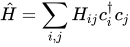
There are ten discrete symmetry classes of topological insulators and superconductors, corresponding to the ten Altland–Zirnbauer classes of random matrices. They are defined by three symmetries of the Hamiltonian ${\displaystyle {\hat {H}}=\sum _{i,j}H_{ij}c_{i}^{\dagger }c_{j}}$, (where ${\displaystyle c_{i}}$, and ${\displaystyle c_{i}^{\dagger }}$, are the annihilation and creation operators of mode ${\displaystyle i}$, in some arbitrary spatial basis) : time-reversal symmetry, particle-hole (or charge conjugation) symmetry, and chiral (or sublattice) symmetry.

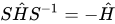
• Chiral symmetry is a unitary operator ${\displaystyle S}$, that acts on ${\displaystyle c_{i}}$, as a unitary rotation (${\displaystyle Sc_{i}S^{-1}=(U_{S})_{ij}c_{j}}$,) and satisfies ${\displaystyle S^{2}=1}$. A Hamiltonian ${\displaystyle H}$ possesses chiral symmetry when ${\displaystyle S{\hat {H}}S^{-1}=-{\hat {H}}}$, for some choice of ${\displaystyle S}$ (on the level of first-quantised Hamiltonians, this means ${\displaystyle U_{S}}$ and ${\displaystyle H}$ are anticommuting matrices).

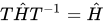
• Time-reversal symmetry (TRS) is an antiunitary operator ${\displaystyle T}$, that acts on ${\displaystyle \alpha c_{i}}$, (where ${\displaystyle \alpha }$, is an arbitrary complex coefficient, and ${\displaystyle ^{*}}$, denotes complex conjugation) as ${\displaystyle T\alpha c_{i}T^{-1}=\alpha ^{*}{(U_{T})}_{ij}c_{j}}$. It can be written as ${\displaystyle T=U_{T}{\mathcal {K}}}$ where ${\displaystyle {\mathcal {K}}}$ is the complex conjugation operator and ${\displaystyle U_{T}}$ is a unitary matrix. Either ${\displaystyle T^{2}=1}$ or ${\displaystyle T^{2}=-1}$. A Hamiltonian with time reversal symmetry satisfies ${\displaystyle T{\hat {H}}T^{-1}={\hat {H}}}$, or on the level of first-quantised matrices, ${\displaystyle U_{T}H^{*}U_{T}^{-1}=H}$, for some choice of ${\displaystyle U_{T}}$.

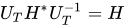
• Charge conjugation or particle-hole symmetry (PHS) ${\displaystyle C}$ is also an antiunitary operator which acts on ${\displaystyle \alpha c_{i}}$ as ${\displaystyle C\alpha c_{i}C^{-1}=\alpha ^{*}(U_{C}^{\dagger })_{ji}c_{j}}$, and can be written as ${\displaystyle C=U_{C}{\mathcal {K}}}$ where ${\displaystyle U_{C}}$ is unitary. Again either ${\displaystyle C^{2}=1}$ or ${\displaystyle C^{2}=-1}$ depending on what ${\displaystyle U_{C}}$ is. A Hamiltonian with particle hole symmetry satisfies ${\displaystyle C{\hat {H}}C^{-1}=-{\hat {H}}}$, or on the level of first-quantised Hamiltonian matrices, ${\displaystyle U_{C}H^{*}U_{C}^{-1}=-H}$, for some choice of ${\displaystyle U_{C}}$.

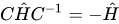
In the Bloch Hamiltonian formalism for crystal structures, where the Hamiltonian ${\displaystyle H(k)}$ acts on modes of crystal momentum ${\displaystyle k}$, the chiral symmetry, TRS, and PHS conditions become

• ${\displaystyle U_{S}H(k)U_{S}^{-1}=-H(k)}$ (chiral symmetry)

• ${\displaystyle U_{T}H(k)^{*}U_{T}^{-1}=H(-k)}$ (time-reversal symmetry),

• ${\displaystyle U_{C}H(k)^{*}U_{C}^{-1}=-H(-k)}$ (particle-hole symmetry).

It is evident that if two of these three symmetries are present, then the third is also present, due to the relation ${\displaystyle S=TC}$.

The aforementioned discrete symmetries label 10 distinct discrete symmetry classes, which coincide with the Altland–Zirnbauer classes of random matrices.

Symmetry class	Time reversal symmetry	Particle hole symmetry	Chiral symmetry
A	No	No	No
AIII	No	No	Yes
AI	Yes, ${\displaystyle T^{2}=1}$	No	No
BDI	Yes, ${\displaystyle T^{2}=1}$	Yes, ${\displaystyle C^{2}=1}$	Yes
D	No	Yes, ${\displaystyle C^{2}=1}$	No
DIII	Yes, ${\displaystyle T^{2}=-1}$	Yes, ${\displaystyle C^{2}=1}$	Yes
AII	Yes, ${\displaystyle T^{2}=-1}$	No	No
CII	Yes, ${\displaystyle T^{2}=-1}$	Yes, ${\displaystyle C^{2}=-1}$	Yes
C	No	Yes, ${\displaystyle C^{2}=-1}$	No
CI	Yes, ${\displaystyle T^{2}=1}$	Yes, ${\displaystyle C^{2}=-1}$	Yes

A bulk Hamiltonian in a particular symmetry group is restricted to be a Hermitian matrix with no zero-energy eigenvalues (i.e. so that the spectrum is "gapped" and the system is a bulk insulator) satisfying the symmetry constraints of the group. In the case of ${\displaystyle d>0}$ dimensions, this Hamiltonian is a continuous function ${\displaystyle H(k)}$ of the ${\displaystyle d}$ parameters in the Bloch momentum vector ${\displaystyle {\vec {k}}}$ in the Brillouin zone; then the symmetry constraints must hold for all ${\displaystyle {\vec {k}}}$.

Given two Hamiltonians ${\displaystyle H_{1}}$ and ${\displaystyle H_{2}}$, it may be possible to continuously deform ${\displaystyle H_{1}}$ into ${\displaystyle H_{2}}$ while maintaining the symmetry constraint and gap (that is, there exists continuous function ${\displaystyle H(t,{\vec {k}})}$ such that for all ${\displaystyle 0\leq t\leq 1}$ the Hamiltonian has no zero eigenvalue and symmetry condition is maintained, and ${\displaystyle H(0,{\vec {k}})=H_{1}({\vec {k}})}$ and ${\displaystyle H(1,{\vec {k}})=H_{2}({\vec {k}})}$). Then we say that ${\displaystyle H_{1}}$ and ${\displaystyle H_{2}}$ are equivalent.

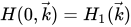
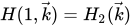
However, it may also turn out that there is no such continuous deformation. in this case, physically if two materials with bulk Hamiltonians ${\displaystyle H_{1}}$ and ${\displaystyle H_{2}}$, respectively, neighbor each other with an edge between them, when one continuously moves across the edge one must encounter a zero eigenvalue (as there is no continuous transformation that avoids this). This may manifest as a gapless zero energy edge mode or an electric current that only flows along the edge.

An interesting question is to ask, given a symmetry class and a dimension of the Brillouin zone, what are all the equivalence classes of Hamiltonians. Each equivalence class can be labeled by a topological invariant; two Hamiltonians whose topological invariant are different cannot be deformed into each other and belong to different equivalence classes.

For each of the symmetry classes, the question can be simplified by deforming the Hamiltonian into a "projective" Hamiltonian, and considering the symmetric space in which such Hamiltonians live. These classifying spaces are shown for each symmetry class:^[4]

Symmetry class	Classifying space	${\displaystyle \pi _{0}}$of Classifying space
A	${\displaystyle \bigcup _{n}\mathrm {U} (N)/(\mathrm {U} (Nn)\times \mathrm {U} (n))}$	${\displaystyle \mathbb {Z} }$
AIII	${\displaystyle \mathrm {U} (N)}$	${\displaystyle 0}$
AI	${\displaystyle \bigcup _{n}\mathrm {O} (N)/(\mathrm {O} (Nn)\times \mathrm {O} (n))}$	${\displaystyle \mathbb {Z} }$
BDI	${\displaystyle \mathrm {O} (N)}$	${\displaystyle \mathbb {Z} _{2}}$
D	${\displaystyle \mathrm {O} (2N)/\mathrm {U} (N)}$	${\displaystyle \mathbb {Z} _{2}}$
DIII	${\displaystyle \mathrm {U} (N)/\mathrm {Sp} (N)}$	${\displaystyle 0}$
AII	${\displaystyle \bigcup _{n}\mathrm {Sp} (N)/(\mathrm {Sp} (Nn)\times \mathrm {Sp} (n))}$	${\displaystyle \mathbb {Z} }$
CII	${\displaystyle \mathrm {Sp} (N)}$	${\displaystyle 0}$
C	${\displaystyle \mathrm {Sp} (2N)/\mathrm {U} (N)}$	${\displaystyle 0}$
CI	${\displaystyle \mathrm {U} (N)/\mathrm {O} (N)}$	${\displaystyle 0}$

For example, a (real symmetric) Hamiltonian in symmetry class AI can have its ${\displaystyle n}$ positive eigenvalues deformed to +1 and its ${\displaystyle Nn}$ negative eigenvalues deformed to -1; the resulting such matrices are described by the union of real Grassmannians${\displaystyle \bigcup _{n=0}^{\infty }\mathrm {Gr} (n,N)=\bigcup _{n=0}^{\infty }\mathrm {O} (N)/\mathrm {\mathrm {O} } (n)\times \mathrm {\mathrm {O} } (Nn)}$

The strong topological invariants of a many-band system in ${\displaystyle d}$ dimensions can be labeled by the elements of the ${\displaystyle d}$-th homotopy group of the symmetric space. These groups are displayed in this table, called the periodic table of topological insulators:

Symmetry class	${\displaystyle d=0}$	${\displaystyle d=1}$	${\displaystyle d=2}$	${\displaystyle d=3}$	${\displaystyle d=4}$	${\displaystyle d=5}$	${\displaystyle d=6}$	${\displaystyle d=7}$	${\displaystyle d=8}$
A	${\displaystyle \mathbb {Z} }$	${\displaystyle 0}$	${\displaystyle \mathbb {Z} }$	${\displaystyle 0}$	${\displaystyle \mathbb {Z} }$	${\displaystyle 0}$	${\displaystyle \mathbb {Z} }$	${\displaystyle 0}$	${\displaystyle \mathbb {Z} }$
AIII	${\displaystyle 0}$	${\displaystyle \mathbb {Z} }$	${\displaystyle 0}$	${\displaystyle \mathbb {Z} }$	${\displaystyle 0}$	${\displaystyle \mathbb {Z} }$	${\displaystyle 0}$	${\displaystyle \mathbb {Z} }$	${\displaystyle 0}$
AI	${\displaystyle \mathbb {Z} }$	${\displaystyle 0}$	${\displaystyle 0}$	${\displaystyle 0}$	${\displaystyle 2\mathbb {Z} }$	${\displaystyle 0}$	${\displaystyle \mathbb {Z} _{2}}$	${\displaystyle \mathbb {Z} _{2}}$	${\displaystyle \mathbb {Z} }$
BDI	${\displaystyle \mathbb {Z} _{2}}$	${\displaystyle \mathbb {Z} }$	${\displaystyle 0}$	${\displaystyle 0}$	${\displaystyle 0}$	${\displaystyle 2\mathbb {Z} }$	${\displaystyle 0}$	${\displaystyle \mathbb {Z} _{2}}$	${\displaystyle \mathbb {Z} _{2}}$
D	${\displaystyle \mathbb {Z} _{2}}$	${\displaystyle \mathbb {Z} _{2}}$	${\displaystyle \mathbb {Z} }$	${\displaystyle 0}$	${\displaystyle 0}$	${\displaystyle 0}$	${\displaystyle 2\mathbb {Z} }$	${\displaystyle 0}$	${\displaystyle \mathbb {Z} _{2}}$
DIII	${\displaystyle 0}$	${\displaystyle \mathbb {Z} _{2}}$	${\displaystyle \mathbb {Z} _{2}}$	${\displaystyle \mathbb {Z} }$	${\displaystyle 0}$	${\displaystyle 0}$	${\displaystyle 0}$	${\displaystyle 2\mathbb {Z} }$	${\displaystyle 0}$
AII	${\displaystyle 2\mathbb {Z} }$	${\displaystyle 0}$	${\displaystyle \mathbb {Z} _{2}}$	${\displaystyle \mathbb {Z} _{2}}$	${\displaystyle \mathbb {Z} }$	${\displaystyle 0}$	${\displaystyle 0}$	${\displaystyle 0}$	${\displaystyle 2\mathbb {Z} }$
CII	${\displaystyle 0}$	${\displaystyle 2\mathbb {Z} }$	${\displaystyle 0}$	${\displaystyle \mathbb {Z} _{2}}$	${\displaystyle \mathbb {Z} _{2}}$	${\displaystyle \mathbb {Z} }$	${\displaystyle 0}$	${\displaystyle 0}$	${\displaystyle 0}$
C	${\displaystyle 0}$	${\displaystyle 0}$	${\displaystyle 2\mathbb {Z} }$	${\displaystyle 0}$	${\displaystyle \mathbb {Z} _{2}}$	${\displaystyle \mathbb {Z} _{2}}$	${\displaystyle \mathbb {Z} }$	${\displaystyle 0}$	${\displaystyle 0}$
CI	${\displaystyle 0}$	${\displaystyle 0}$	${\displaystyle 0}$	${\displaystyle 2\mathbb {Z} }$	${\displaystyle 0}$	${\displaystyle \mathbb {Z} _{2}}$	${\displaystyle \mathbb {Z} _{2}}$	${\displaystyle \mathbb {Z} }$	${\displaystyle 0}$

There may also exist weak topological invariants (associated to the fact that the suspension of the Brillouin zone is in fact equivalent to a ${\displaystyle d+1}$ sphere wedged with lower-dimensional spheres), which are not included in this table. Furthermore, the table assumes the limit of an infinite number of bands, i.e. involves ${\displaystyle N\times N}$ Hamiltonians for ${\displaystyle N\to \infty }$.

The table also is periodic in the sense that the group of invariants in ${\displaystyle d}$ dimensions is the same as the group of invariants in ${\displaystyle d+8}$ dimensions. In the case of no anti-unitary symmetries, the invariant groups are periodic in dimension by 2.

For nontrivial symmetry classes, the actual invariant can be defined by one of the following integrals over all or part of the Brillouin zone: the Chern number, the Wess-Zuminowinding number, the Chern–Simons invariant, the Fu–Kane invariant.

The periodic table also displays a peculiar property: the invariant groups in ${\displaystyle d}$ dimensions are identical to those in ${\displaystyle d-1}$ dimensions but in a different symmetry class. Among the complex symmetry classes, the invariant group for A in ${\displaystyle d}$ dimensions is the same as that for AIII in ${\displaystyle d-1}$ dimensions, and vice versa. One can also imagine arranging each of the eight real symmetry classes on the Cartesian plane such that the ${\displaystyle x}$ coordinate is ${\displaystyle T^{2}}$ if time reversal symmetry is present and ${\displaystyle 0}$ if it is absent, and the ${\displaystyle y}$ coordinate is ${\displaystyle C^{2}}$ if particle hole symmetry is present and ${\displaystyle 0}$ if it is absent. Then the invariant group in ${\displaystyle d}$ dimensions for a certain real symmetry class is the same as the invariant group in ${\displaystyle d-1}$ dimensions for the symmetry class directly one space clockwise. This phenomenon was termed the Bott clock by Alexei Kitaev, in reference to the Bott periodicity theorem.^[1][10]

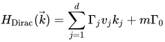
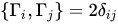
The Bott clock can be understood by considering the problem of Clifford algebra extensions.^[1] Near an interface between two inequivalent bulk materials, the Hamiltonian approaches a gap closing. To lowest order expansion in momentum slightly away from the gap closing, the Hamiltonian takes the form of a Dirac Hamiltonian ${\displaystyle H_{\text{Dirac}}({\vec {k}})=\sum _{j=1}^{d}\Gamma _{j}v_{j}k_{j}+m\Gamma _{0}}$. Here, ${\displaystyle \Gamma _{1},\Gamma _{2},\ldots ,\Gamma _{d}}$ are a representation of the Clifford Algebra ${\displaystyle \lbrace \Gamma _{i},\Gamma _{j}\rbrace =2\delta _{ij}}$, while ${\displaystyle m\Gamma _{0}}$هو "مصطلح كتلة" إضافي يتبادل عكسيًا مع بقية الهاميلتوني ويتلاشى عند السطح البيني (مما يعطي السطح البيني نمط حافة بدون فجوة عند${\displaystyle k=0}$). ال${\displaystyle m\Gamma _{0}}$لا يمكن تشويه مصطلح الهاميلتوني على أحد جانبي الواجهة بشكل مستمر إلى${\displaystyle m\Gamma _{0}}$مصطلح للهاميلتوني على الجانب الآخر من السطح البيني. وبالتالي (بفرض${\displaystyle m}$(ليكن عددًا قياسيًا موجبًا اختياريًا) فإن مشكلة تصنيف الثوابت الطوبولوجية تختزل إلى مشكلة تصنيف جميع الخيارات غير المتكافئة الممكنة لـ${\displaystyle \Gamma _{0}}$لتوسيع جبر كليفورد إلى بُعد أعلى واحد، مع الحفاظ على قيود التناظر.