
Stationary state
A stationary state is a quantum state with all observables independent of time. It is an eigenvector of the energy operator (instead of a quantum superposition of different energies). It is also called energy eigenvector, energy eigenstate, energy eigenfunction, or energy eigenket. It is very similar to the concept of atomic orbital and molecular orbital in chemistry, with some slight differences explained below.
Introduction
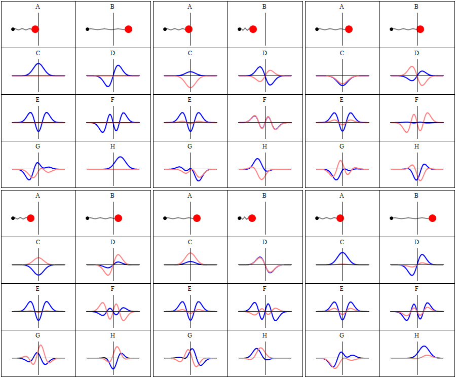
A stationary state is called stationary because the system remains in the same state as time elapses, in every observable way. For a single-particle Hamiltonian, this means that the particle has a constant probability distribution for its position, its velocity, its spin, etc.[1] (This is true assuming the particle's environment is also static, i.e. the Hamiltonian is unchanging in time.) The wavefunction itself is not stationary: It continually changes its overall complex phase factor, so as to form a standing wave. The oscillation frequency of the standing wave, multiplied by the Planck constant, is the energy of the state according to the Planck–Einstein relation.
Stationary states are quantum states that are solutions to the time-independent Schrödinger equation: where
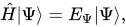
- is a quantum state, which is a stationary state if it satisfies this equation;
- is the Hamiltonian operator;
- is a real number, and corresponds to the energy eigenvalue of the state .


This is an eigenvalue equation: is a linear operator on a vector space, is an eigenvector of , and is its eigenvalue.
If a stationary state is plugged into the time-dependent Schrödinger equation, the result is[2]
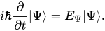
Assuming that is time-independent (unchanging in time), this equation holds for any time t. Therefore, this is a differential equation describing how varies in time. Its solution is

Therefore, a stationary state is a standing wave that oscillates with an overall complex phase factor, and its oscillation angular frequency is equal to its energy divided by .

Stationary state properties
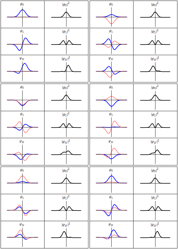

As shown above, a stationary state is not mathematically constant:
However, all observable properties of the state are in fact constant in time. For example, if represents a simple one-dimensional single-particle wavefunction , the probability that the particle is at location x is which is independent of the time t.



The Heisenberg picture is an alternative mathematical formulation of quantum mechanics where stationary states are truly mathematically constant in time.
As mentioned above, these equations assume that the Hamiltonian is time-independent. This means simply that stationary states are only stationary when the rest of the system is fixed and stationary as well. For example, a 1s electron in a hydrogen atom is in a stationary state, but if the hydrogen atom reacts with another atom, then the electron will of course be disturbed.
Spontaneous decay
Spontaneous decay complicates the question of stationary states. For example, according to simple (nonrelativistic) quantum mechanics, the hydrogen atom has many stationary states: 1s, 2s, 2p, and so on, are all stationary states. But in reality, only the ground state 1s is truly "stationary": An electron in a higher energy level will spontaneously emit one or more photons to decay into the ground state.[3] This seems to contradict the idea that stationary states should have unchanging properties.
يكمن التفسير في أن الهاميلتوني المستخدم في ميكانيكا الكم غير النسبية ليس إلا تقريبًا للهاميلتوني المُستمد من نظرية الحقل الكمومي . تُعتبر حالات الإلكترون ذات الطاقة الأعلى (2s، 2p، 3s، إلخ) حالات مستقرة وفقًا للهاميلتوني التقريبي، ولكنها ليست مستقرة وفقًا للهاميلتوني الحقيقي، وذلك بسبب تقلبات الفراغ . من ناحية أخرى، تُعد حالة 1s حالة مستقرة بالفعل، وفقًا لكلٍ من الهاميلتوني التقريبي والحقيقي.
مقارنة بـ "المدار" في الكيمياء
المدار هو حالة مستقرة (أو تقريب لها) لذرة أو جزيء يحتوي على إلكترون واحد؛ وبشكل أكثر تحديدًا، هو مدار ذري لإلكترون في ذرة، أو مدار جزيئي لإلكترون في جزيء. [ 4 ]
بالنسبة لجزيء يحتوي على إلكترون واحد فقط (مثل ذرة الهيدروجين أو H₂⁺ ) ، فإن المدار هو نفسه الحالة المستقرة الكلية للجزيء. أما بالنسبة لجزيء متعدد الإلكترونات، فإن المدار يختلف تمامًا عن الحالة المستقرة الكلية، التي تمثل حالة متعددة الجسيمات تتطلب وصفًا أكثر تعقيدًا (مثل محدد سلاتر ). [ 5 ] على وجه الخصوص، في جزيء متعدد الإلكترونات، لا يمثل المدار الحالة المستقرة الكلية للجزيء، بل يمثل الحالة المستقرة لإلكترون واحد داخل الجزيء. ويكون مفهوم المدار هذا ذا معنى فقط في ظل التقريب التالي: إذا تجاهلنا حدود التنافر اللحظي بين الإلكترونات في الهاميلتوني كفرضية تبسيطية، فيمكننا تحليل المتجه الذاتي الكلي لجزيء متعدد الإلكترونات إلى مساهمات منفصلة من حالات الإلكترونات المستقرة (المدارات)، والتي يتم الحصول على كل منها في ظل تقريب الإلكترون الواحد. (لحسن الحظ، يمكن للكيميائيين والفيزيائيين في كثير من الأحيان (ولكن ليس دائمًا) استخدام "تقريب الإلكترون الواحد" هذا.) بهذا المعنى، في نظام متعدد الإلكترونات، يمكن اعتبار المدار بمثابة الحالة الثابتة لإلكترون فردي في النظام.
في الكيمياء، يفترض حساب المدارات الجزيئية عادةً تقريب بورن-أوبنهايمر .
انظر أيضاً
مراجع
- ↑ كلود كوهين-تانوجي ، وبرنارد ديو، وفرانك لالوي . ميكانيكا الكم: المجلد الأول . هيرمان، 1977. ص 32.
- ↑ الكميات: دليل للمفاهيم، بقلم ب . و. أتكينز، مطبعة جامعة أكسفورد، 1974، رقم ISBN 0-19-855493-1.
- ↑ فيزياء الكم للذرات والجزيئات والمواد الصلبة والنوى والجسيمات (الطبعة الثانية)، ر. إيسبرغ، ر. ريسنيك، جون وايلي وأولاده، 1985، رقم ISBN 978-0-471-87373-0
- ↑ الكيمياء الفيزيائية، بقلم ب . و. أتكينز، مطبعة جامعة أكسفورد، 1978، رقم ISBN 0-19-855148-7.
- ↑ لودين، بير-أولوف (1955). "النظرية الكمية لأنظمة الجسيمات المتعددة. الجزء الأول: التفسيرات الفيزيائية باستخدام مصفوفات الكثافة، والمدارات الدورانية الطبيعية، ومسائل التقارب في طريقة التفاعل التكويني". مجلة Physical Review ، 97 (6): 1474-1489 . Bibcode : 1955PhRv...97.1474L . doi : 10.1103/PhysRev.97.1474 .
للمزيد من القراءة
- الحالات المستقرة ، آلان هولدن، مطبعة جامعة أكسفورد، 1971، رقم ISBN 0-19-851121-3
- ميكانيكا الكم