Flory–Huggins solution theory

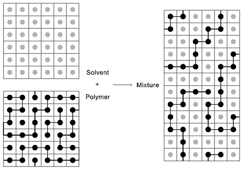
Flory–Huggins solution theory is a lattice model of the thermodynamics of polymer solutions which takes account of the great dissimilarity in molecular sizes in adapting the usual expression for the entropy of mixing. The result is an equation for the Gibbs free energy change ${\displaystyle \Delta G_{\rm {mix}}}$ for mixing a polymer with a solvent. Although it makes simplifying assumptions, it generates useful results for interpreting experiments.

The theory is named after Paul Flory and Maurice Loyal Huggins who developed it independently in 1941.

The thermodynamic equation for the Gibbs energy change accompanying mixing at constant temperature and (external) pressure is

${\displaystyle \Delta G_{\rm {mix}}=\Delta H_{\rm {mix}}-T\Delta S_{\rm {mix}}}$

A change, denoted by ${\displaystyle \Delta }$, is the value of a variable for a solution or mixture minus the values for the pure components considered separately. The objective is to find explicit formulas for ${\displaystyle \Delta H_{\rm {mix}}}$ and ${\displaystyle \Delta S_{\rm {mix}}}$, the enthalpy and entropy increments associated with the mixing process.

The result obtained by Flory and Huggins is

${\displaystyle \Delta G_{\rm {mix}}=RT[\,n_{1}\ln \phi _{1}+n_{2}\ln \phi _{2}+n_{1}\phi _{2}\chi _{12}\,]}$

The right-hand side is a function of the number of moles${\displaystyle n_{1}}$ and volume fraction ${\displaystyle \phi _{1}}$ of solvent (component ${\displaystyle 1}$), the number of moles ${\displaystyle n_{2}}$ and volume fraction ${\displaystyle \phi _{2}}$ of polymer (component ${\displaystyle 2}$), with the introduction of a parameter ${\displaystyle \chi }$ to take account of the energy of interdispersing polymer and solvent molecules. ${\displaystyle R}$ is the gas constant and ${\displaystyle T}$ is the absolute temperature. The volume fraction is analogous to the mole fraction, but is weighted to take account of the relative sizes of the molecules. For a small solute, the mole fractions would appear instead, and this modification is the innovation due to Flory and Huggins. In the most general case the mixing parameter, ${\displaystyle \chi }$, is a free energy parameter, thus including an entropic component.^[1][2]

We first calculate the entropy of mixing, the increase in the uncertainty about the locations of the molecules when they are interspersed. In the pure condensed phases – solvent and polymer – a molecule exists for any arbitrarily small volume element. The expression for the entropy of mixing of small molecules in terms of mole fractions is no longer reasonable when the solute is a macromolecularchain. We take account of this dissymmetry in molecular sizes by assuming that individual polymer segments and individual solvent molecules occupy sites on a lattice. Each site is occupied by exactly one molecule of the solvent or by one monomer of the polymer chain, so the total number of sites is

${\displaystyle N=N_{1}+xN_{2}}$

where ${\displaystyle N_{1}}$ is the number of solvent molecules and ${\displaystyle N_{2}}$ is the number of polymer molecules, each of which has ${\displaystyle x}$ segments.

For a random walk on a lattice^[3] we can calculate the entropy change (the increase in spatialuncertainty) as a result of mixing solute and solvent.

${\displaystyle \Delta S_{\rm {mix}}=-k_{\rm {B}}\left[N_{1}\ln {\tfrac {N_{1}}{N}}+N_{2}\ln {\tfrac {xN_{2}}{N}}\right]}$

where ${\displaystyle k_{\rm {B}}}$ is the Boltzmann constant. Define the lattice volume fractions${\displaystyle \phi _{1}}$ and ${\displaystyle \phi _{2}}$

${\displaystyle \phi _{1}={\frac {N_{1}}{N}},\quad \phi _{2}={\frac {xN_{2}}{N}}}$

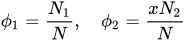
These are also the probabilities that a given lattice site, chosen at random, is occupied by a solvent molecule or a polymer segment, respectively. Thus

${\displaystyle \Delta S_{\rm {mix}}=-k_{\rm {B}}[\,N_{1}\ln \phi _{1}+N_{2}\ln \phi _{2}\,]}$

For a small solute whose molecules occupy just one lattice site, ${\displaystyle x}$ equals one, the volume fractions reduce to molecular or mole fractions, and we recover the usual entropy of mixing.

In addition to the entropic effect, we can expect an enthalpy change. There are three molecular interactions to consider: solvent-solvent ${\displaystyle w_{11}}$, monomer-monomer ${\displaystyle w_{22}}$ (not the covalent bonding, but between different chain sections), and monomer-solvent ${\displaystyle w_{12}}$. Each of the last occurs at the expense of the average of the other two, so the energy increment per monomer-solvent contact is

${\displaystyle \Delta w=w_{12}-{\tfrac {1}{2}}(w_{22}+w_{11})}$

The total number of such contacts is

${\displaystyle xN_{2}z\phi _{1}=N_{1}\phi _{2}z}$

where ${\displaystyle z}$ is the coordination number, the number of nearest neighbors for a lattice site, each one occupied either by one chain segment or a solvent molecule. That is, ${\displaystyle xN_{2}}$ is the total number of polymer segments (monomers) in the solution, so ${\displaystyle xN_{2}z}$ is the number of nearest-neighbor sites to all the polymer segments. Multiplying by the probability ${\displaystyle \phi _{1}}$ that any such site is occupied by a solvent molecule, we obtain the total number of polymer-solvent molecular interactions. An approximation following mean field theory is made by following this procedure, thereby reducing the complex problem of many interactions to a simpler problem of one interaction.

The enthalpy change is equal to the energy change per polymer monomer-solvent interaction multiplied by the number of such interactions

${\displaystyle \Delta H_{\rm {mix}}=N_{1}\phi _{2}z\Delta w}$

The polymer-solvent interaction parameter chi is defined as

${\displaystyle \chi _{12}={\frac {z\Delta w}{k_{\rm {B}}T}}}$

It depends on the nature of both the solvent and the solute, and is the only material-specific parameter in the model. The enthalpy change becomes

${\displaystyle \Delta H_{\rm {mix}}=k_{\rm {B}}TN_{1}\phi _{2}\chi _{12}}$

Assembling terms, the total free energy change is

${\displaystyle \Delta G_{\rm {mix}}=RT[\,n_{1}\ln \phi _{1}+n_{2}\ln \phi _{2}+n_{1}\phi _{2}\chi _{12}\,]}$

where we have converted the expression from molecules ${\displaystyle N_{1}}$ and ${\displaystyle N_{2}}$ to moles ${\displaystyle n_{1}}$ and ${\displaystyle n_{2}}$ by transferring the Avogadro constant${\displaystyle N_{\text{A}}}$ to the gas constant${\displaystyle R=k_{\rm {B}}N_{\text{A}}}$.

The value of the interaction parameter can be estimated from the Hildebrand solubility parameters${\displaystyle \delta _{a}}$ and ${\displaystyle \delta _{b}}$

${\displaystyle \chi _{12}={\frac {V_{\rm {seg}}(\delta _{a}-\delta _{b})^{2}}{RT}}}$

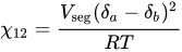
where ${\displaystyle V_{\rm {seg}}}$ is the actual volume of a polymer segment.

In the most general case the interaction ${\displaystyle \Delta w}$ and the ensuing mixing parameter, ${\displaystyle \chi }$, is a free energy parameter, thus including an entropic component.^[1][2] The Flory–Huggins interaction parameter χ represents the energetic interaction between polymer segments and solvent molecules. It reflects the difference between polymer–solvent interactions and the average interactions of polymer–polymer and solvent–solvent pairs. Larger positive values of χ indicate unfavorable mixing and may lead to phase separation, whereas smaller values correspond to better miscibility. In many polymer–solvent systems the parameter is temperature dependent and often decreases as temperature increases.^[4] This means that aside to the regular mixing entropy there is another entropic contribution from the interaction between solvent and monomer. This contribution is sometimes very important in order to make quantitative predictions of thermodynamic properties.

More advanced solution theories exist, such as the Flory–Krigbaum theory.

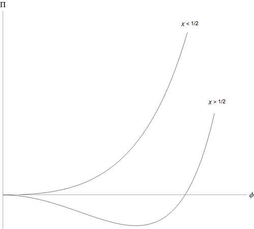
Polymers can separate out from the solvent, and do so in a characteristic way.^[5] The Flory–Huggins free energy per unit volume, for a polymer with ${\displaystyle N}$ monomers, can be written in a simple dimensionless form

${\displaystyle f={\frac {\phi }{N}}\ln \phi +(1-\phi )\ln(1-\phi )+\chi \phi (1-\phi )}$

for ${\displaystyle \phi }$ the volume fraction of monomers, and ${\displaystyle N\gg 1}$. The osmotic pressure (in reduced units) is

${\displaystyle \Pi ={\frac {\phi }{N}}-\ln(1-\phi )-\phi -\chi \phi ^{2}}$.

The polymer solution is stable with respect to small fluctuations when the second derivative of this free energy is positive. This second derivative is

${\displaystyle f''={\frac {1}{N\phi }}+{\frac {1}{1-\phi }}-2\chi }$

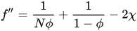
and the solution first becomes unstable when this and the third derivative

${\displaystyle f'''=-{\frac {1}{N\phi ^{2}}}+{\frac {1}{(1-\phi )^{2}}}}$

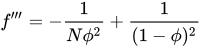
are both equal to zero. A little algebra then shows that the polymer solution first becomes unstable at a critical point at

${\displaystyle \chi _{\text{cp}}\simeq 1/2+N^{-1/2}+\cdots \qquad \phi _{\text{cp}}\simeq N^{-1/2}-N^{-1}+\cdots }$

This means that for all values of ${\displaystyle 0<\chi \lesssim 1/2}$ the monomer-solvent effective interaction is weakly repulsive, but this is too weak to cause liquid/liquid separation. However, when ${\displaystyle \chi >1/2}$, there is separation into two coexisting phases, one richer in polymer but poorer in solvent, than the other.

The unusual feature of the liquid/liquid phase separation is that it is highly asymmetric: the volume fraction of monomers at the critical point is approximately ${\displaystyle N^{-1/2}}$, which is very small for large polymers. The amount of polymer in the solvent-rich/polymer-poor coexisting phase is extremely small for long polymers. The solvent-rich phase is close to pure solvent. This is peculiar to polymers, a mixture of small molecules can be approximated using the Flory–Huggins expression with ${\displaystyle N=1}$, and then ${\displaystyle \phi _{\text{cp}}=1/2}$ and both coexisting phases are far from pure.

Synthetic polymers rarely consist of chains of uniform length in solvent. The Flory–Huggins free energy density can be generalized^[6] to an N-component mixture of polymers with lengths ${\displaystyle r_{i}}$ by

${\displaystyle f{\Bigl (}\{\phi _{i},r_{i}\}{\Bigr )}=\sum _{i=1}^{N}{\frac {\phi _{i}}{r_{i}}}\ln \phi _{i}+{\frac {1}{2}}\sum _{i,j=1}^{N}\phi _{i}\phi _{j}\chi _{ij}}$

For a binary polymer blend, where one species consists of ${\displaystyle N_{A}}$ monomers and the other ${\displaystyle N_{B}}$ monomers this simplifies to

${\displaystyle f(\phi )={\frac {\phi }{N_{A}}}\ln \phi +{\frac {1-\phi }{N_{B}}}\ln(1-\phi )+\chi \phi (1-\phi )}$

As in the case for dilute polymer solutions, the first two terms on the right-hand side represent the entropy of mixing. For large polymers of ${\displaystyle N_{A}\gg 1}$ and ${\displaystyle N_{B}\gg 1}$ these terms are negligibly small. This implies that for a stable mixture to exist ${\displaystyle \chi <0}$, so for polymers A and B to blend their segments must attract one another.^[7]

Flory–Huggins theory tends to agree well with experiments in the semi-dilute concentration regime and can be used to fit data for even more complicated blends with higher concentrations. The theory qualitatively predicts phase separation, the tendency for high molecular weight species to be immiscible, the ${\displaystyle \chi \propto T^{-1}}$ interaction-temperature dependence and other features commonly observed in polymer mixtures. However, unmodified Flory–Huggins theory fails to predict the lower critical solution temperature observed in some polymer blends and the lack of dependence of the critical temperature ${\displaystyle T_{\text{c}}}$ on chain length ${\displaystyle r_{i}}$.^[8] Additionally, it can be shown that for a binary blend of polymer species with equal chain lengths ${\displaystyle (N_{A}=N_{B})}$ the critical concentration should be ${\displaystyle \psi _{\text{c}}=1/2}$; however, polymers blends have been observed where this parameter is highly asymmetric. In certain blends, mixing entropy can dominate over monomer interaction. By adopting the mean-field approximation, ${\displaystyle \chi }$ parameter complex dependence on temperature, blend composition, and chain length was discarded. Specifically, interactions beyond the nearest neighbor may be highly relevant to the behavior of the blend and the distribution of polymer segments is not necessarily uniform, so certain lattice sites may experience interaction energies disparate from that approximated by the mean-field theory.

One well-studied^[5][7] effect on interaction energies neglected by unmodified Flory–Huggins theory is chain correlation. In dilute polymer mixtures, where chains are well separated, intramolecular forces between monomers of the polymer chain dominate and drive demixing leading to regions where polymer concentration is high. As the polymer concentration increases, chains tend to overlap and the effect becomes less important. In fact, the demarcation between dilute and semi-dilute solutions is commonly defined by the concentration where polymers begin to overlap ${\displaystyle c^{*}}$ which can be estimated as

${\displaystyle c^{*}={\frac {m}{{\frac {4}{3}}\pi R_{\text{g}}^{3}}}}$

Here, m is the mass of a single polymer chain, and ${\displaystyle R_{\text{g}}}$ is the chain's radius of gyration.

• "Conformations, Solutions and Molecular Weight" (book chapter), Chapter 3 of Book Title: Polymer Science and Technology; by Joel R. Fried; 2nd Edition, 2003

References

- 12Burchard, W (1983). "Solution Thermodyanmics of Non-Ionic Water Soluble Polymers.". In Finch, C. (ed.). Chemistry and Technology of Water-Soluble Polymers. Springer. pp. 125–142. ISBN 978-1-4757-9661-2.
- 12Franks, F (1983). "Water Solubility and Sensitivity-Hydration Effects.". In Finch, C. (ed.). Chemistry and Technology of Water-Soluble Polymers. Springer. pp. 157–178. ISBN 978-1-4757-9661-2.
- ↑Dijk, Menno A. van; Wakker, Andre (1998-01-14). Concepts in Polymer Thermodynamics. CRC Press. pp. 61–65. ISBN 978-1-56676-623-4.
- ↑Rubinstein, Michael; Colby, Ralph H. (2003). Polymer Physics. Oxford University Press. ISBN 9780198520597.
- 12de Gennes, Pierre-Gilles (1979). Scaling concepts in polymer physics. Ithaca, N.Y.: Cornell University Press. ISBN 080141203X. OCLC 4494721.
- ↑Berry, J; et al. (2018). "Physical principles of intracellular organization via active and passive phase transitions". Reports on Progress in Physics. 81 (46601): 046601. Bibcode:2018RPPh...81d6601B. doi:10.1088/1361-6633/aaa61e. PMID 29313527. S2CID 4039711.
- 12Doi, Masao (2013). Soft Matter Physics. Great Clarendon Street, Oxford, UK: Oxford University Press. ISBN 9780199652952.
- ↑Schmid, Friederike (2010). "Theory and Simulation of Multiphase Polymer Systems". arXiv:1001.1265 [cond-mat.soft].
External links