
Finite strain theory
In continuum mechanics, the finite strain theory—also called large strain theory, or large deformation theory—deals with deformations in which strains and/or rotations are large enough to invalidate assumptions inherent in infinitesimal strain theory. In this case, the undeformed and deformed configurations of the continuum are significantly different, requiring a clear distinction between them. This is commonly the case with elastomers, plastically deforming materials and other fluids and biologicalsoft tissue.
Displacement field
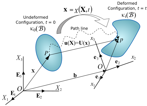
The displacement of a body has two components: a rigid-body displacement and a deformation.
- A rigid-body displacement consists of a translation and rotation of the body without changing its shape or size.
- Deformation implies the change in shape and/or size of the body from an initial or undeformed configuration to a current or deformed configuration (Figure 1).


A change in the configuration of a continuum body can be described by a displacement field. A displacement field is a vector field of all displacement vectors for all particles in the body, which relates the deformed configuration with the undeformed configuration. The distance between any two particles changes if and only if deformation has occurred. If displacement occurs without deformation, then it is a rigid-body displacement.
Deformation gradient tensor

The deformation gradient tensor is a quantity related to both the reference and current configuration, and expresses motion locally around a point. Two types of deformation gradient tensor may be defined.
The material deformation gradient tensor is a second-order tensor that represents the gradient of the smooth and invertible mapping function , which describes the motion of a continuum. In particular, the continuity of the mapping function implies that cracks and voids do not open or close during the deformation. The material deformation gradient tensor characterizes the local deformation at a material point with position vector , i.e., deformation at neighbouring points, by transforming (linear transformation) a material line element emanating from that point from the reference configuration to the current or deformed configuration. Thus we have,



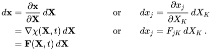
Assuming that has a smooth inverse, has the inverse , which is the spatial deformation gradient tensor. being invertible is equivalent to , which corresponds to the notion that the material cannot be infinitely compressed.


Relative displacement vector
Consider a particle or material point with position vector in the undeformed configuration (Figure 2). After a displacement of the body, the new position of the particle indicated by in the new configuration is given by the vector position . The coordinate systems for the undeformed and deformed configuration can be superimposed for convenience.


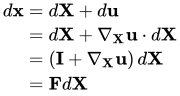
Consider now a material point neighboring , with position vector . In the deformed configuration this particle has a new position given by the position vector . Assuming that the line segments and joining the particles and in both the undeformed and deformed configuration, respectively, to be very small, then we can express them as and . Thus from Figure 2 we have





where is the relative displacement vector, which represents the relative displacement of with respect to in the deformed configuration.

Taylor approximation
For an infinitesimal element , and assuming continuity on the displacement field, it is possible to use a Taylor series expansion around point , neglecting higher-order terms, to approximate the components of the relative displacement vector for the neighboring particle as Thus, the previous equation can be written as



Time-derivative of the deformation gradient
Calculations that involve the time-dependent deformation of a body often require a time derivative of the deformation gradient to be calculated. A geometrically consistent definition of such a derivative requires an excursion into differential geometry[1] but we avoid those issues in this article.
The time derivative of is where is the (material) velocity. The derivative on the right hand side represents a material velocity gradient. It is common to convert that into a spatial gradient by applying the chain rule for derivatives, i.e., where is the spatial velocity gradient and where is the spatial (Eulerian) velocity at . If the spatial velocity gradient is constant in time, the above equation can be solved exactly to give assuming at . There are several methods of computing the exponential above.
![{\displaystyle {\dot {\mathbf {F} }}={\frac {\partial \mathbf {F} }{\partial t}}={\frac {\partial }{\partial t}}\left[{\frac {\partial \mathbf {x} (\mathbf {X} ,t)}{\partial \mathbf {X} }}\right]={\frac {\partial }{\partial \mathbf {X} }}\left[{\frac {\partial \mathbf {x} (\mathbf {X} ,t)}{\partial t}}\right]={\frac {\partial }{\partial \mathbf {X} }}\left[\mathbf {V} (\mathbf {X} ,t)\right]}](https://wikimedia.org/api/rest_v1/media/math/render/svg/f2666606a9db3c727de1e94fa372b590683f72c0)

![{\displaystyle {\dot {\mathbf {F} }}={\frac {\partial }{\partial \mathbf {X} }}\left[\mathbf {V} (\mathbf {X} ,t)\right]={\frac {\partial }{\partial \mathbf {X} }}\left[\mathbf {v} (\mathbf {x} (\mathbf {X} ,t),t)\right]=\left.{\frac {\partial }{\partial \mathbf {x} }}\left[\mathbf {v} (\mathbf {x} ,t)\right]\right|_{\mathbf {x} =\mathbf {x} (\mathbf {X} ,t)}\cdot {\frac {\partial \mathbf {x} (\mathbf {X} ,t)}{\partial \mathbf {X} }}={\boldsymbol {l}}\cdot \mathbf {F} }](https://wikimedia.org/api/rest_v1/media/math/render/svg/abbb3bd21a0c39cedc504214b5bb20503386c081)




Related quantities often used in continuum mechanics are the rate of deformation tensor and the spin tensor defined, respectively, as: The rate of deformation tensor gives the rate of stretching of line elements while the spin tensor indicates the rate of rotation or vorticity of the motion.

The material time derivative of the inverse of the deformation gradient (keeping the reference configuration fixed) is often required in analyses that involve finite strains. This derivative is The above relation can be verified by taking the material time derivative of and noting that .



Polar decomposition of the deformation gradient tensor
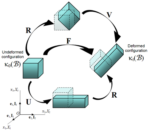
The deformation gradient , like any invertible second-order tensor, can be decomposed, using the polar decomposition theorem, into a product of two second-order tensors (Truesdell and Noll, 1965): an orthogonal tensor and a positive definite symmetric tensor, i.e., where the tensor is a proper orthogonal tensor, i.e., and , representing a rotation; the tensor is the right stretch tensor; and the left stretch tensor. The terms right and left means that they are to the right and left of the rotation tensor , respectively. and are both positive definite, i.e. and for all non-zero , and symmetric tensors, i.e. and , of second order.






This decomposition implies that the deformation of a line element in the undeformed configuration onto in the deformed configuration, i.e., , may be obtained either by first stretching the element by , i.e. , followed by a rotation , i.e., ; or equivalently, by applying a rigid rotation first, i.e., , followed later by a stretching , i.e., (See Figure 3).


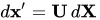


Due to the orthogonality of so that and have the same eigenvalues or principal stretches, but different eigenvectors or principal directions and , respectively. The principal directions are related by



This polar decomposition, which is unique as is invertible with a positive determinant, is a corollary of the singular-value decomposition.
Transformation of a surface and volume element
To transform quantities that are defined with respect to areas in a deformed configuration to those relative to areas in a reference configuration, and vice versa, we use Nanson's relation, expressed as where is an area of a region in the deformed configuration, is the same area in the reference configuration, and is the outward normal to the area element in the current configuration while is the outward normal in the reference configuration, is the deformation gradient, and .



The corresponding formula for the transformation of the volume element is








Fundamental strain tensors
A strain tensor is defined by the IUPAC as:[3]
"A symmetric tensor that results when a deformation gradient tensor is factorized into a rotation tensor followed or preceded by a symmetric tensor".
Since a pure rotation should not induce any strains in a deformable body, it is often convenient to use rotation-independent measures of deformation in continuum mechanics. As a rotation followed by its inverse rotation leads to no change () we can exclude the rotation by multiplying the deformation gradient tensor by its transpose.

Several rotation-independent deformation gradient tensors (or "deformation tensors", for short) are used in mechanics. In solid mechanics, the most popular of these are the right and left Cauchy–Green deformation tensors.
Cauchy strain tensor (right Cauchy–Green deformation tensor)
In 1839, George Green introduced a deformation tensor known as the right Cauchy–Green deformation tensor or Green's deformation tensor (the IUPAC recommends that this tensor be called the Cauchy strain tensor),[3] defined as:

Physically, the Cauchy–Green tensor gives us the square of local change in distances due to deformation, i.e.

Invariants of are often used in the expressions for strain energy density functions. The most commonly used invariants are where is the determinant of the deformation gradient and are stretch ratios for the unit fibers that are initially oriented along the eigenvector directions of the right (reference) stretch tensor (these are not generally aligned with the three axis of the coordinate systems).

![{\displaystyle {\begin{aligned}I_{1}^{C}&:={\text{tr}}(\mathbf {C} )=C_{II}=\lambda _{1}^{2}+\lambda _{2}^{2}+\lambda _{3}^{2}\\I_{2}^{C}&:={\tfrac {1}{2}}\left[({\text{tr}}~\mathbf {C} )^{2}-{\text{tr}}(\mathbf {C} ^{2})\right]={\tfrac {1}{2}}\left[(C_{JJ})^{2}-C_{IK}C_{KI}\right]=\lambda _{1}^{2}\lambda _{2}^{2}+\lambda _{2}^{2}\lambda _{3}^{2}+\lambda _{3}^{2}\lambda _{1}^{2}\\I_{3}^{C}&:=\det(\mathbf {C} )=J^{2}=\lambda _{1}^{2}\lambda _{2}^{2}\lambda _{3}^{2}.\end{aligned}}}](https://wikimedia.org/api/rest_v1/media/math/render/svg/6d05cca3762fe510c6252312cb22a66da138cfef)


Finger strain tensor
The IUPAC recommends[3] that the inverse of the right Cauchy–Green deformation tensor (called the Cauchy strain tensor in that document), i. e., , be called the Finger strain tensor. However, that nomenclature is not universally accepted in applied mechanics.


Green strain tensor (left Cauchy–Green deformation tensor)
Reversing the order of multiplication in the formula for the right Cauchy-Green deformation tensor leads to the left Cauchy–Green deformation tensor which is defined as:

The left Cauchy–Green deformation tensor is often called the Finger deformation tensor, named after Josef Finger (1894).[4]
The IUPAC recommends that this tensor be called the Green strain tensor.[3]
Invariants of are also used in the expressions for strain energy density functions. The conventional invariants are defined as where is the determinant of the deformation gradient.

![{\displaystyle {\begin{aligned}I_{1}&:={\text{tr}}(\mathbf {B} )=B_{ii}=\lambda _{1}^{2}+\lambda _{2}^{2}+\lambda _{3}^{2}\\I_{2}&:={\tfrac {1}{2}}\left[({\text{tr}}~\mathbf {B} )^{2}-{\text{tr}}(\mathbf {B} ^{2})\right]={\tfrac {1}{2}}\left(B_{ii}^{2}-B_{jk}B_{kj}\right)=\lambda _{1}^{2}\lambda _{2}^{2}+\lambda _{2}^{2}\lambda _{3}^{2}+\lambda _{3}^{2}\lambda _{1}^{2}\\I_{3}&:=\det \mathbf {B} =J^{2}=\lambda _{1}^{2}\lambda _{2}^{2}\lambda _{3}^{2}\end{aligned}}}](https://wikimedia.org/api/rest_v1/media/math/render/svg/7e88d7c726ee801990cc0dda3221b4a2edc04aa5)
For compressible materials, a slightly different set of invariants is used:

Piola strain tensor (Cauchy deformation tensor)
Earlier in 1828,[5]Augustin-Louis Cauchy introduced a deformation tensor defined as the inverse of the left Cauchy–Green deformation tensor, . This tensor has also been called the Piola strain tensor by the IUPAC[3] and the Finger tensor[6] in the rheology and fluid dynamics literature.


Spectral representation
If there are three distinct principal stretches , the spectral decompositions of and is given by


Furthermore,


Observe that Therefore, the uniqueness of the spectral decomposition also implies that . The left stretch () is also called the spatial stretch tensor while the right stretch () is called the material stretch tensor.


The effect of acting on is to stretch the vector by and to rotate it to the new orientation , i.e., In a similar vein,


Examples
- Uniaxial extension of an incompressible material
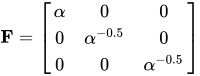
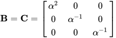
- This is the case where a specimen is stretched in 1-direction with a stretch ratio of . If the volume remains constant, the contraction in the other two directions is such that or . Then:
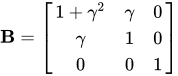
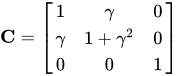
- Simple shear
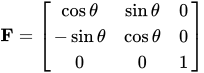
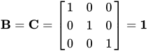
- Rigid body rotation




Derivatives of stretch
Derivatives of the stretch with respect to the right Cauchy–Green deformation tensor are used to derive the stress-strain relations of many solids, particularly hyperelastic materials. These derivatives are and follow from the observations that :(\mathbf {N} _{i}\otimes \mathbf {N} _{i})=\lambda _{i}^{2}~;~~~~{\cfrac {\partial \mathbf {C} }{\partial \mathbf {C} }}={\mathsf {I}}^{(s)}~;~~~~{\mathsf {I}}^{(s)}:(\mathbf {N} _{i}\otimes \mathbf {N} _{i})=\mathbf {N} _{i}\otimes \mathbf {N} _{i}.}


Physical interpretation of deformation tensors
Let be a Cartesian coordinate system defined on the undeformed body and let be another system defined on the deformed body. Let a curve in the undeformed body be parametrized using . Its image in the deformed body is .


![{\displaystyle s\in [0,1]}](https://wikimedia.org/api/rest_v1/media/math/render/svg/aff1a54fbbee4a2677039524a5139e952fa86eb9)

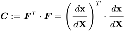
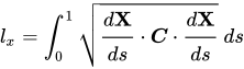
The undeformed length of the curve is given by After deformation, the length becomes Note that the right Cauchy–Green deformation tensor is defined as Hence, which indicates that changes in length are characterized by .

![{\displaystyle {\begin{aligned}l_{x}&=\int _{0}^{1}\left|{\cfrac {d\mathbf {x} }{ds}}\right|~ds=\int _{0}^{1}{\sqrt {{\cfrac {d\mathbf {x} }{ds}}\cdot {\cfrac {d\mathbf {x} }{ds}}}}~ds=\int _{0}^{1}{\sqrt {\left({\cfrac {d\mathbf {x} }{d\mathbf {X} }}\cdot {\cfrac {d\mathbf {X} }{ds}}\right)\cdot \left({\cfrac {d\mathbf {x} }{d\mathbf {X} }}\cdot {\cfrac {d\mathbf {X} }{ds}}\right)}}~ds\\&=\int _{0}^{1}{\sqrt {{\cfrac {d\mathbf {X} }{ds}}\cdot \left[\left({\cfrac {d\mathbf {x} }{d\mathbf {X} }}\right)^{T}\cdot {\cfrac {d\mathbf {x} }{d\mathbf {X} }}\right]\cdot {\cfrac {d\mathbf {X} }{ds}}}}~ds\end{aligned}}}](https://wikimedia.org/api/rest_v1/media/math/render/svg/dd1b639bab0e25d96cf46894973e1d2693800d94)

Finite strain tensors
The concept of strain is used to evaluate how much a given displacement differs locally from a rigid body displacement.[7][8][9] One of such strains for large deformations is the Lagrangian finite strain tensor, also called the Green-Lagrangian strain tensor or Green–St-Venant strain tensor, defined as

or as a function of the displacement gradient tensor or
![{\displaystyle \mathbf {E} ={\frac {1}{2}}\left[(\nabla _{\mathbf {X} }\mathbf {u} )^{T}+\nabla _{\mathbf {X} }\mathbf {u} +(\nabla _{\mathbf {X} }\mathbf {u} )^{T}\cdot \nabla _{\mathbf {X} }\mathbf {u} \right]}](https://wikimedia.org/api/rest_v1/media/math/render/svg/613f67ee25337f305e0fe930e90f5099becdc913)

The Green-Lagrangian strain tensor is a measure of how much differs from .

The Eulerian finite strain tensor, or Eulerian-Almansi finite strain tensor, referenced to the deformed configuration (i.e. Eulerian description) is defined as

or as a function of the displacement gradients we have

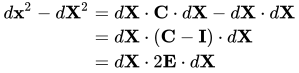
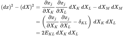
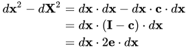
A measure of deformation is the difference between the squares of the differential line element , in the undeformed configuration, and , in the deformed configuration (Figure 2). Deformation has occurred if the difference is non zero, otherwise a rigid-body displacement has occurred. Thus we have,

In the Lagrangian description, using the material coordinates as the frame of reference, the linear transformation between the differential lines is

Then we have,

where are the components of the right Cauchy–Green deformation tensor, . Then, replacing this equation into the first equation we have,


or where , are the components of a second-order tensor called the Green – St-Venant strain tensor or the Lagrangian finite strain tensor,

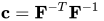
In the Eulerian description, using the spatial coordinates as the frame of reference, the linear transformation between the differential lines is where are the components of the spatial deformation gradient tensor, . Thus we have



where the second order tensor is called Cauchy's deformation tensor, . Then we have,


or
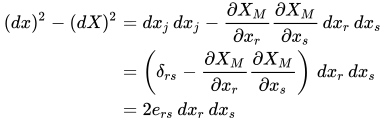
where , are the components of a second-order tensor called the Eulerian-Almansi finite strain tensor,


Both the Lagrangian and Eulerian finite strain tensors can be conveniently expressed in terms of the displacement gradient tensor. For the Lagrangian strain tensor, first we differentiate the displacement vector with respect to the material coordinates to obtain the material displacement gradient tensor,


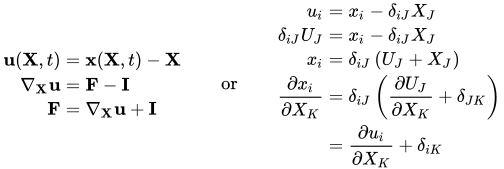
Replacing this equation into the expression for the Lagrangian finite strain tensor we have or
![{\displaystyle {\begin{aligned}\mathbf {E} &={\frac {1}{2}}\left(\mathbf {F} ^{T}\mathbf {F} -\mathbf {I} \right)\\&={\frac {1}{2}}\left[\left\{(\nabla _{\mathbf {X} }\mathbf {u} )^{T}+\mathbf {I} \right\}\left(\nabla _{\mathbf {X} }\mathbf {u} +\mathbf {I} \right)-\mathbf {I} \right]\\&={\frac {1}{2}}\left[(\nabla _{\mathbf {X} }\mathbf {u} )^{T}+\nabla _{\mathbf {X} }\mathbf {u} +(\nabla _{\mathbf {X} }\mathbf {u} )^{T}\cdot \nabla _{\mathbf {X} }\mathbf {u} \right]\\\end{aligned}}}](https://wikimedia.org/api/rest_v1/media/math/render/svg/a1bc4d02e18262b73b16470e4e4cfb36c933410b)
![{\displaystyle {\begin{aligned}E_{KL}&={\frac {1}{2}}\left({\frac {\partial x_{j}}{\partial X_{K}}}{\frac {\partial x_{j}}{\partial X_{L}}}-\delta _{KL}\right)\\&={\frac {1}{2}}\left[\delta _{jM}\left({\frac {\partial U_{M}}{\partial X_{K}}}+\delta _{MK}\right)\delta _{jN}\left({\frac {\partial U_{N}}{\partial X_{L}}}+\delta _{NL}\right)-\delta _{KL}\right]\\&={\frac {1}{2}}\left[\delta _{MN}\left({\frac {\partial U_{M}}{\partial X_{K}}}+\delta _{MK}\right)\left({\frac {\partial U_{N}}{\partial X_{L}}}+\delta _{NL}\right)-\delta _{KL}\right]\\&={\frac {1}{2}}\left[\left({\frac {\partial U_{M}}{\partial X_{K}}}+\delta _{MK}\right)\left({\frac {\partial U_{M}}{\partial X_{L}}}+\delta _{ML}\right)-\delta _{KL}\right]\\&={\frac {1}{2}}\left({\frac {\partial U_{K}}{\partial X_{L}}}+{\frac {\partial U_{L}}{\partial X_{K}}}+{\frac {\partial U_{M}}{\partial X_{K}}}{\frac {\partial U_{M}}{\partial X_{L}}}\right)\end{aligned}}}](https://wikimedia.org/api/rest_v1/media/math/render/svg/8613306031cc1580236c979b6aec6c795d3e4db9)
Similarly, the Eulerian-Almansi finite strain tensor can be expressed as
Seth–Hill family of generalized strain tensors
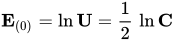
B. R. Seth from the Indian Institute of Technology Kharagpur was the first to show that the Green and Almansi strain tensors are special cases of a more general strain measure.[10][11] The idea was further expanded upon by Rodney Hill in 1968.[12] The Seth–Hill family of strain measures (also called Doyle-Ericksen tensors)[13] can be expressed as
![{\displaystyle \mathbf {E} _{(m)}={\frac {1}{2m}}(\mathbf {U} ^{2m}-\mathbf {I} )={\frac {1}{2m}}\left[\mathbf {C} ^{m}-\mathbf {I} \right]}](https://wikimedia.org/api/rest_v1/media/math/render/svg/70e3f0b7ddba558d16a401580cf534133ef24d09)
For different values of we have:

- Green-Lagrangian strain tensor
- Biot strain tensor
- Logarithmic strain, Natural strain, True strain, or Hencky strain
- Almansi strain


![{\displaystyle \mathbf {E} _{(-1)}={\frac {1}{2}}\left[\mathbf {I} -\mathbf {U} ^{-2}\right]}](https://wikimedia.org/api/rest_v1/media/math/render/svg/0446d9edf116c655919b58ac4fc46fab8778af99)
The second-order approximation of these tensors is where is the infinitesimal strain tensor.


Many other different definitions of tensors are admissible, provided that they all satisfy the conditions that:[14]

- vanishes for all rigid-body motions
- the dependence of on the displacement gradient tensor is continuous, continuously differentiable and monotonic
- it is also desired that reduces to the infinitesimal strain tensor as the norm


An example is the set of tensors which do not belong to the Seth–Hill class, but have the same 2nd-order approximation as the Seth–Hill measures at for any value of .[15]



Physical interpretation of the finite strain tensor
The diagonal components of the Lagrangian finite strain tensor are related to the normal strain, e.g.

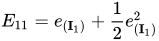
where is the normal strain or engineering strain in the direction .


The off-diagonal components of the Lagrangian finite strain tensor are related to shear strain, e.g.

where is the change in the angle between two line elements that were originally perpendicular with directions and , respectively.


Under certain circumstances, i.e. small displacements and small displacement rates, the components of the Lagrangian finite strain tensor may be approximated by the components of the infinitesimal strain tensor
The stretch ratio for the differential element (Figure) in the direction of the unit vector at the material point , in the undeformed configuration, is defined as


where is the deformed magnitude of the differential element .

Similarly, the stretch ratio for the differential element (Figure), in the direction of the unit vector at the material point , in the deformed configuration, is defined as


The square of the stretch ratio is defined as
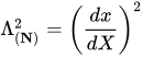
Knowing that we have where and are unit vectors.




The normal strain or engineering strain in any direction can be expressed as a function of the stretch ratio,


Thus, the normal strain in the direction at the material point may be expressed in terms of the stretch ratio as
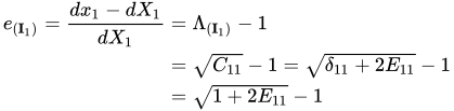
solving for we have

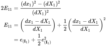
The shear strain, or change in angle between two line elements and initially perpendicular, and oriented in the principal directions and , respectively, can also be expressed as a function of the stretch ratio. From the dot product between the deformed lines and we have


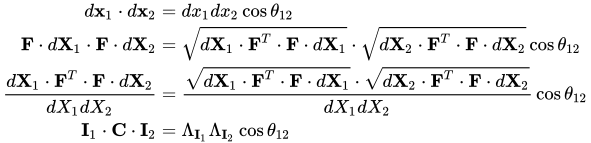
where is the angle between the lines and in the deformed configuration. Defining as the shear strain or reduction in the angle between two line elements that were originally perpendicular, we have

thus, then
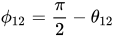


or
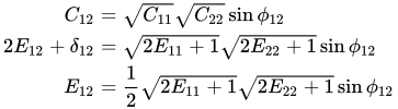
Compatibility conditions
The problem of compatibility in continuum mechanics involves the determination of allowable single-valued continuous fields on bodies. These allowable conditions leave the body without unphysical gaps or overlaps after a deformation. Most such conditions apply to simply-connected bodies. Additional conditions are required for the internal boundaries of multiply connected bodies.
Compatibility of the deformation gradient
The necessary and sufficient conditions for the existence of a compatible field over a simply connected body are


Compatibility of the right Cauchy–Green deformation tensor
The necessary and sufficient conditions for the existence of a compatible field over a simply connected body are We can show these are the mixed components of the Riemann–Christoffel curvature tensor. Therefore, the necessary conditions for -compatibility are that the Riemann–Christoffel curvature of the deformation is zero.
![{\displaystyle R_{\alpha \beta \rho }^{\gamma }:={\frac {\partial }{\partial X^{\rho }}}[\,_{(X)}\Gamma _{\alpha \beta }^{\gamma }]-{\frac {\partial }{\partial X^{\beta }}}[\,_{(X)}\Gamma _{\alpha \rho }^{\gamma }]+\,_{(X)}\Gamma _{\mu \rho }^{\gamma }\,_{(X)}\Gamma _{\alpha \beta }^{\mu }-\,_{(X)}\Gamma _{\mu \beta }^{\gamma }\,_{(X)}\Gamma _{\alpha \rho }^{\mu }=0}](https://wikimedia.org/api/rest_v1/media/math/render/svg/29e1d54640569dc6ab58c0fca0c0ab634aef2180)
Compatibility of the left Cauchy–Green deformation tensor
General sufficiency conditions for the left Cauchy–Green deformation tensor in three dimensions has been discussed in several works.[16]
See also
- Infinitesimal strain
- Compatibility (mechanics)
- Curvilinear coordinates
- Piola–Kirchhoff stress tensor, the stress tensor for finite deformations.
- Stress measures
- Strain partitioning
References
- ↑A. Yavari, J.E. Marsden, and M. Ortiz, On spatial and material covariant balance laws in elasticity, Journal of Mathematical Physics, 47, 2006, 042903; pp. 1–53.
- ↑Eduardo de Souza Neto; Djordje Peric; Owens, David (2008). Computational methods for plasticity : theory and applications. Chichester, West Sussex, UK: Wiley. p. 65. ISBN 978-0-470-69452-7.
- 12345A. Kaye, R. F. T. Stepto, W. J. Work, J. V. Aleman (Spain), A. Ya. Malkin (1998). "Definition of terms relating to the non-ultimate mechanical properties of polymers". Pure Appl. Chem. 70 (3): 701–754. doi:10.1351/pac199870030701.
{{cite journal}}: CS1 maint: multiple names: authors list (link) - ↑Eduardo N. Dvorkin, Marcela B. Goldschmit, 2006 Nonlinear Continua, p. 25, Springer ISBN 3-540-24985-0.
- ↑Jirásek,Milan; Bažant, Z. P. (2002) Inelastic analysis of structures, Wiley, p. 463 ISBN 0-471-98716-6
- ↑J. N. Reddy, David K. Gartling (2000) The finite element method in heat transfer and fluid dynamics, p. 317, CRC Press ISBN 1-4200-8598-0.
- ↑Lubliner, Jacob (2008). Plasticity Theory(PDF) (Revised ed.). Dover Publications. ISBN 978-0-486-46290-5. Archived from the original(PDF) on 2010-03-31.
- ↑Belytschko, Ted; Liu, Wing Kam; Moran, Brian (2000). Nonlinear Finite Elements for Continua and Structures (reprint with corrections, 2006 ed.). John Wiley & Sons Ltd. pp. 92–94. ISBN 978-0-471-98773-4.
- ↑Zeidi, Mahdi; Kim, Chun IL (2018). "Mechanics of an elastic solid reinforced with bidirectional fiber in finite plane elastostatics: complete analysis". Continuum Mechanics and Thermodynamics. 30 (3): 573–592. Bibcode:2018CMT....30..573Z. doi:10.1007/s00161-018-0623-0. ISSN 1432-0959. S2CID 253674037.
- ↑Seth, B. R. (1961), "Generalized strain measure with applications to physical problems", MRC Technical Summary Report #248, Mathematics Research Center, United States Army, University of Wisconsin: 1–18, archived from the original on August 22, 2013
- ↑Seth, B. R. (1962), "Generalized strain measure with applications to physical problems", IUTAM Symposium on Second Order Effects in Elasticity, Plasticity and Fluid Mechanics, Haifa, 1962.
- ↑Hill, R. (1968), "On constitutive inequalities for simple materials—I", Journal of the Mechanics and Physics of Solids, 16 (4): 229–242, Bibcode:1968JMPSo..16..229H, doi:10.1016/0022-5096(68)90031-8
- ↑T.C. Doyle and J.L. Eriksen (1956). "Non-linear elasticity." Advances in Applied Mechanics 4, 53–115.
- ↑Z.P. Bažant and L. Cedolin (1991). Stability of Structures. Elastic, Inelastic, Fracture and Damage Theories. Oxford Univ. Press, New York (2nd ed. Dover Publ., New York 2003; 3rd ed., World Scientific 2010).
- ↑Z.P. Bažant (1998). "Easy-to-compute tensors with symmetric inverse approximating Hencky finite strain and its rate." Journal of Materials of Technology ASME, 120 (April), 131–136.
- ↑Acharya, A. (1999). "On Compatibility Conditions for the Left Cauchy–Green Deformation Field in Three Dimensions"(PDF). Journal of Elasticity. 56 (2): 95–105. doi:10.1023/A:1007653400249. S2CID 116767781.; Blume, J. A. (1989). "Compatibility conditions for a left Cauchy–Green strain field". Journal of Elasticity. 21 (3): 271–308. doi:10.1007/BF00045780. S2CID 54889553.
Further reading
- Dill, Ellis Harold (2006). Continuum Mechanics: Elasticity, Plasticity, Viscoelasticity. Germany: CRC Press. ISBN 0-8493-9779-0.
- Dimitrienko, Yuriy (2011). Nonlinear Continuum Mechanics and Large Inelastic Deformations. Germany: Springer. ISBN 978-94-007-0033-8.
- Hutter, Kolumban; Klaus Jöhnk (2004). Continuum Methods of Physical Modeling. Germany: Springer. ISBN 3-540-20619-1.
- Lubarda, Vlado A. (2001). Elastoplasticity Theory. CRC Press. ISBN 0-8493-1138-1.
- Macosko, C. W. (1994). Rheology: principles, measurement and applications. VCH Publishers. ISBN 1-56081-579-5.
- Mase, George E. (1970). Continuum Mechanics. McGraw-Hill Professional. ISBN 0-07-040663-4.
- Mase, G. Thomas; George E. Mase (1999). Continuum Mechanics for Engineers (Second ed.). CRC Press. ISBN 0-8493-1855-6.
- Nemat-Nasser, Sia (2006). Plasticity: A Treatise on Finite Deformation of Heterogeneous Inelastic Materials. Cambridge: Cambridge University Press. ISBN 0-521-83979-3.
- Rees, David (2006). Basic Engineering Plasticity – An Introduction with Engineering and Manufacturing Applications. Butterworth-Heinemann. ISBN 0-7506-8025-3.
External links
- Tensors
- Continuum mechanics
- Elasticity (physics)
- Non-Newtonian fluids
- Solid mechanics