
Laplace distribution
In probability theory and statistics, the Laplace distribution is a continuous probability distribution named after Pierre-Simon Laplace. It is also sometimes called the double exponential distribution, because it can be thought of as two exponential distributions (with an additional location parameter) spliced together along the x-axis,[1] although the term is also sometimes used to refer to the Gumbel distribution. The difference between two independent identically distributed exponential random variables is governed by a Laplace distribution, as is a Brownian motion evaluated at an exponentially distributed random time. Increments of Laplace motion or a variance gamma process evaluated over the time scale also have a Laplace distribution.
Definitions
Probability density function
A random variable has a distribution if its probability density function is
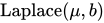

where is a location parameter, and , which is sometimes referred to as the "diversity", is a scale parameter. If and , the positive half-line is exactly an exponential distribution scaled by 1/2.[2]


The probability density function of the Laplace distribution is also reminiscent of the normal distribution; however, whereas the normal distribution is expressed in terms of the squared difference from the mean , the Laplace density is expressed in terms of the absolute difference from the mean. Consequently, the Laplace distribution has fatter tails than the normal distribution. It is a special case of the generalized normal distribution and the hyperbolic distribution. Continuous symmetric distributions that have exponential tails, like the Laplace distribution, but which have probability density functions that are differentiable at the mode include the logistic distribution, hyperbolic secant distribution, and the Champernowne distribution.
Cumulative distribution function
The Laplace distribution is easy to integrate (if one distinguishes two symmetric cases) due to the use of the absolute value function. Its cumulative distribution function is as follows:
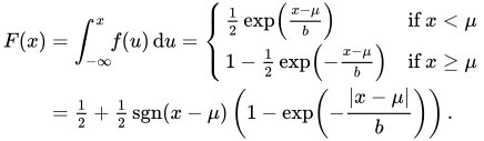
The inverse cumulative distribution function is given by

Properties
Moments
![{\displaystyle \mu _{r}'={\frac {1}{2}}\sum _{k=0}^{r}\left[{\frac {r!}{(rk)!}}b^{k}\mu ^{(rk)}\left\{1+(-1)^{k}\right\}\right].}](https://wikimedia.org/api/rest_v1/media/math/render/svg/d094efa4a1e7355825cc9b032028c43732c830c3)
Related distributions
- If then .
- If then .
- If then (exponential distribution).
- If then .
- If then .
- If then (exponential power distribution).
- If (normal distribution) then and .
- If then (chi-squared distribution).
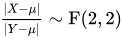
- If then . (F-distribution)
- If (uniform distribution) then .
- If and (Bernoulli distribution) independent of , then .
- If and independent of , then .
- If has a Rademacher distribution and then .
- If and independent of , then .
- If (geometric stable distribution) then .
- The Laplace distribution is a limiting case of the hyperbolic distribution.
- If with (Rayleigh distribution) then . Note that if , then with , which in turn equals the exponential distribution .
- Given an integer , if (gamma distribution, using characterization), then (infinite divisibility)[3]
- If X has a Laplace distribution, then Y = eX has a log-Laplace distribution; conversely, if X has a log-Laplace distribution, then its logarithm has a Laplace distribution.



































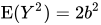
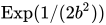

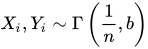


Probability of a Laplace being greater than another
Let be independent laplace random variables: and , and we want to compute .




The probability of can be reduced (using the properties below) to , where . This probability is equal to



When , both expressions are replaced by their limit as :


To compute the case for , note that


since when .


Relation to the exponential distribution
A Laplace random variable can be represented as the difference of two independent and identically distributed (iid) exponential random variables.[3] One way to show this is by using the characteristic function approach. For any set of independent continuous random variables, for any linear combination of those variables, its characteristic function (which uniquely determines the distribution) can be acquired by multiplying the corresponding characteristic functions.
Consider two i.i.d random variables . The characteristic functions for are


respectively. On multiplying these characteristic functions (equivalent to the characteristic function of the sum of the random variables ), the result is

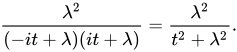
This is the same as the characteristic function for , which is


Sargan distributions
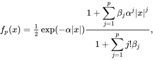
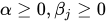
Sargan distributions are a system of distributions of which the Laplace distribution is a core member. A th order Sargan distribution has density[4][5] for parameters . The Laplace distribution results for .


Statistical inference
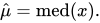
Given independent and identically distributed samples , the maximum likelihood (MLE) estimator of is the sample median,[6]


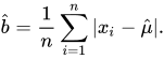
The MLE estimator of is the mean absolute deviation from the median, revealing a link between the Laplace distribution and least absolute deviations. A correction for small samples can be applied as follows: (see: exponential distribution#Parameter estimation).


Occurrence and applications
The Laplacian distribution has been used in speech recognition to model priors on DFT coefficients [7] and in JPEG image compression to model AC coefficients [8] generated by a DCT.
- The addition of noise drawn from a Laplacian distribution, with scaling parameter appropriate to a function's sensitivity, to the output of a statistical database query is the most common means to provide differential privacy in statistical databases.

- In regression analysis, the least absolute deviations estimate arises as the maximum likelihood estimate if the errors have a Laplace distribution.
- The Lasso can be thought of as a Bayesian regression with a Laplacian prior for the coefficients.[9]
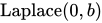
- In hydrology the Laplace distribution is applied to extreme events such as annual maximum one-day rainfalls and river discharges. The blue picture illustrates an example of fitting the Laplace distribution to ranked annually maximum one-day rainfalls showing also the 90% confidence belt based on the binomial distribution. The rainfall data are represented by plotting positions as part of the cumulative frequency analysis.
- يُستخدم توزيع لابلاس في مجال التمويل. فعلى سبيل المثال، طوّر إس جي كو نموذجًا لأسعار الأدوات المالية يتضمن توزيع لابلاس (وفي بعض الحالات توزيع لابلاس غير متماثل ) لمعالجة مشاكل الالتواء والتفرطح وابتسامة التقلب التي غالبًا ما تحدث عند استخدام التوزيع الطبيعي لتسعير هذه الأدوات. [ 10 ] [ 11 ]
- يُعد توزيع لابلاس، كونه توزيعًا مركبًا أو مزدوجًا ، قابلاً للتطبيق في الحالات التي تنشأ فيها القيم الدنيا في ظل ظروف خارجية مختلفة عن القيم العليا، بحيث تتبع نمطًا مختلفًا. [ 12 ]
توليد المتغيرات العشوائية
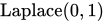
بافتراض وجود متغير عشوائيتم سحبها من التوزيع المنتظم في الفترةالمتغير العشوائي



له توزيع لابلاس بمعاملاتووهذا يتبع من دالة التوزيع التراكمي العكسي المذكورة أعلاه.
أيمكن أيضًا إنشاء المتغير كفرق بين متغيرين مستقلين ومتطابقين في التوزيع.المتغيرات العشوائية. أو بصورة مكافئة،ويمكن أيضًا توليدها كلوغاريتم نسبة متغيرين عشوائيين مستقلين ومتطابقين وموزعين توزيعًا منتظمًا.

تاريخ
يُشار إلى هذا التوزيع غالبًا باسم "قانون لابلاس الأول للأخطاء". وقد نشره عام 1774، حيث صوّر تكرار الخطأ كدالة أسية لقيمته بمجرد تجاهل إشارته. لاحقًا، استبدل لابلاس هذا النموذج بـ"قانونه الثاني للأخطاء"، المستند إلى التوزيع الطبيعي، بعد اكتشاف نظرية النهاية المركزية . [ 13 ] [ 14 ]
نشر كينز ورقة بحثية في عام 1911 استنادًا إلى أطروحته السابقة حيث أظهر أن توزيع لابلاس يقلل من الانحراف المطلق عن الوسيط. [ 15 ]
انظر أيضاً
- التوزيع الطبيعي المعمم#النسخة المتماثلة
- توزيع لابلاس متعدد المتغيرات
- مقياس بيسوف ، وهو تعميم لتوزيع لابلاس إلى فضاءات الدوال
- توزيع كوشي ، ويسمى أيضًا "توزيع لورنتزيان"، أي تحويل فورييه لتوزيع لابلاس
- الدالة المميزة (نظرية الاحتمالات)
- دالة من نوع 1s Slater ، تُستخدم في الكيمياء الكمومية
مراجع
- ↑ تشاتامفيلي، راجان؛ شانموغام، رامالينغام (2021)، "توزيع لابلاس" ، التوزيعات المستمرة في الهندسة والعلوم التطبيقية - الجزء الثاني ، تشام: دار نشر سبرينغر الدولية، ص 189-199 ، doi : 10.1007/978-3-031-02435-1_4 ، ISBN 978-3-031-01307-2تم الاطلاع عليه بتاريخ 2025-04-04
- ↑ هوانغ، يونفي؛ وآخرون (2022). "الاستدلال المتفرق والتعلم النشط للمعادلات التفاضلية العشوائية من البيانات" . التقارير العلمية . 12 (1): 21691. arXiv : 2203.11010 . Bibcode : 2022NatSR..1221691H . doi : 10.1038/ s41598-022-25638-9 . PMC 9755218. PMID 36522347 .
- 1 2 كوتز، صموئيل؛ كوزوبوفسكي، توماش ج.؛ بودغورسكي، كريستوف (2001). توزيع لابلاس وتعميماته: إعادة نظر مع تطبيقات في الاتصالات والاقتصاد والهندسة والتمويل . بيركهاوزر. ص 23 (الفرضية 2.2.2، المعادلة 2.2.8). ISBN 9780817641665.
- ↑ إيفريت، بي إس (2002) قاموس كامبريدج للإحصاء ، مطبعة جامعة كامبريدج. رقم ISBN 0-521-81099-X
- ↑ جونسون، إن إل، كوتز، إس، بالاكريشنان، إن (1994) التوزيعات أحادية المتغير المستمرة ، وايلي. ISBN 0-471-58495-9ص 60
- ↑ روبرت م. نورتون (مايو 1984). "التوزيع الأسي المزدوج: استخدام حساب التفاضل والتكامل لإيجاد مُقدِّر الاحتمال الأقصى". الإحصائي الأمريكي . 38 (2). الجمعية الإحصائية الأمريكية: 135-136 . doi : 10.2307/2683252 . JSTOR 2683252 .
- ↑ إلتوفت، ت.؛ تايسو كيم؛ تي-وون لي (2006). "حول توزيع لابلاس متعدد المتغيرات" (ملف PDF) . رسائل معالجة الإشارات IEEE . 13 (5): 300-303 . رمز Bibcode : 2006ISPL...13..300E . doi : 10.1109/LSP.2006.870353 . S2CID 1011487. مؤرشف من الأصل (ملف PDF) بتاريخ 2013-06-06 . تم الاسترجاع بتاريخ 2012-07-04 .
- ↑ مينغيلون، ج.؛ بوجول، ج. (2001). "نمذجة خطأ التكميم الموحد لمعيار JPEG مع تطبيقات على أوضاع التشغيل التسلسلي والتدريجي" (ملف PDF) . مجلة التصوير الإلكتروني . 10 (2): 475-485 . Bibcode : 2001JEI....10..475M . doi : 10.1117/1.1344592 . hdl : 10609/6263 .
- ↑ باردو، سكوت (2020). التحليل الإحصائي لأساليب البيانات التجريبية في العلوم التطبيقية . سبرينغر. ص 58. ISBN 978-3-030-43327-7.
- ↑ كو، إس جي (8 أغسطس 2002). "نموذج الانتشار القفزي لتسعير الخيارات" . مجلة علوم الإدارة . 48 (8): 1086-1101 . doi : 10.1287/mnsc.48.8.1086.166 . JSTOR 822677. تاريخ الاسترجاع: 1 مارس 2022 .
- ↑ تشين، جيان (2018). طريقة تسعير خيارات التوازن العام: دراسة نظرية وتجريبية . سبرينغر. ص 70. ISBN 9789811074288.
- ↑ مجموعة من التوزيعات المركبة
- ^ لابلاس، ملاحظة. (1774). احتفظ باحتمالية الأسباب للأحداث. مذكرات الأكاديمية الملكية للعلوم المقدمة للغواصين سافان، 6، 621-656
- ↑ ويلسون، إدوين بيدويل (1923). "القانونان الأول والثاني للخطأ". مجلة الجمعية الإحصائية الأمريكية . 18 (143). إنفورما المملكة المتحدة المحدودة: 841-851 . doi : 10.1080/01621459.1923.10502116 . ISSN 0162-1459 .
 تتضمن هذه المقالة نصًا من هذا المصدر، وهو متاح للعموم .
 - ↑ كينز، ج. م. (1911). "المتوسطات الرئيسية وقوانين الخطأ المؤدية إليها" . مجلة الجمعية الإحصائية الملكية . 74 (3). JSTOR: 322–331 . doi : 10.2307/2340444 . ISSN 0952-8385 . JSTOR 2340444 .
روابط خارجية
- "توزيع لابلاس" ، موسوعة الرياضيات ، دار نشر EMS ، 2001 [1994]
- التوزيعات المستمرة
- توزيعات الاحتمالية المركبة
- بيير سيمون لابلاس
- توزيعات العائلة الأسية
- توزيعات احتمالية عائلية على مستوى الموقع
- التوزيعات الهندسية المستقرة
- توزيعات احتمالية قابلة للقسمة بلا حدود