Gröbner basis

In mathematics, and more specifically in computer algebra, computational algebraic geometry, and computational commutative algebra, a Gröbner basis is a particular kind of generating set of an ideal in a polynomial ring $K[x_{1},\ldots ,x_{n}]$ over a field $K$ . A Gröbner basis allows many important properties of the ideal and the associated algebraic variety to be deduced easily, such as the dimension and the number of zeros when it is finite. Gröbner basis computation is one of the main practical tools for solving systems of polynomial equations and computing the images of algebraic varieties under projections or rational maps.

Gröbner basis computation can be seen as a multivariate, non-linear generalization of both Euclid's algorithm for computing polynomial greatest common divisors, and Gaussian elimination for linear systems.^[1]

Gröbner bases were introduced by Bruno Buchberger in his 1965 Ph.D. thesis, which also included an algorithm to compute them (Buchberger's algorithm). He named them after his advisor Wolfgang Gröbner. In 2007, Buchberger received the Association for Computing Machinery's Paris Kanellakis Theory and Practice Award for this work. However, the Russian mathematician Nikolai Günther had introduced a similar notion in 1913, published in various Russian mathematical journals. These papers were largely ignored by the mathematical community until their rediscovery in 1987 by Bodo Renschuch et al.^[2] An analogous concept for multivariate power series was developed independently by Heisuke Hironaka in 1964, who named them standard bases. This term has been used by some authors to also denote Gröbner bases.

The theory of Gröbner bases has been extended by many authors in various directions. It has been generalized to other structures such as polynomials over principal ideal rings or polynomial rings, and also some classes of non-commutative rings and algebras, like Ore algebras.

Tools

Polynomial ring

Gröbner bases are primarily defined for ideals in a polynomial ring $R=K[x_{1},\ldots ,x_{n}]$ على حقل $K.$ على الرغم من أن النظرية تعمل لأي حقل، إلا أن معظم حسابات أساس جروبنر تتم إما عندما يكون $K$ هو حقل الأعداد النسبية أو الأعداد الصحيحة modulo عدد أولي.

في سياق قواعد غروبنر، متعددة الحدود غير الصفرية في $R=K[x_{1},\ldots ,x_{n}]$ يُعبَّر عنه عادةً كمجموع $c_{1}M_{1}+\cdots +c_{m}M_{m},$ حيث $c_{i}$ هي عناصر غير صفرية من $K$ ، وتسمى المعاملات ، و $M_{i}$ هي أحاديات (يطلق عليها بوخبيرغر وبعض أتباعه اسم منتجات القوى ) من الشكل $x_{1}^{a_{1}}\cdots x_{n}^{a_{n}},$ حيث $a_{i}$ هي أعداد صحيحة غير سالبة. المتجه $A=[a_{1},\ldots ,a_{n}]$ يُطلق عليه اسم متجه الأس للحد الأحادي. عندما تكون القائمة $X=[x_{1},\ldots ,x_{n}]$ عندما تكون المتغيرات ثابتة، غالبًا ما يتم اختصار ترميز أحاديات الحدود إلى $x_{1}^{a_{1}}\cdots x_{n}^{a_{n}}=X^{A}.$

تُعرَّف أحاديات الحدود تعريفًا فريدًا بواسطة متجهات أسسها، وعند تحديد ترتيب أحاديات الحدود (انظر أدناه)، يُمثَّل كثير الحدود تمثيلًا فريدًا بواسطة قائمة مرتبة من الأزواج المرتبة التي تتكون من متجه الأسس والمعامل المقابل. يُعد هذا التمثيل لكثيرات الحدود فعالًا للغاية لحساب أساس غروبنر في الحواسيب، على الرغم من أنه أقل ملاءمةً لحسابات أخرى مثل تحليل كثير الحدود إلى عوامله الأولية وإيجاد القاسم المشترك الأكبر لكثير الحدود .

لو $F=\{f_{1},\ldots ,f_{k}\}$ هي مجموعة منتهية من كثيرات الحدود في حلقة كثيرات الحدود $R$ ، والمثالي المتولد بواسطة $F$ هو مجموعة التراكيب الخطية لعناصر $F$ ذات المعاملات في $R$ ؛ أي مجموعة كثيرات الحدود التي يمكن كتابتها ${\textstyle \sum _{i=1}^{k}g_{i}f_{i}}$ مع $g_{1},\ldots ,g_{k}\in R.$

ترتيب أحادي الحد

تتطلب جميع العمليات المتعلقة بقواعد غروبنر اختيار ترتيب كلي على أحاديات الحدود، مع خصائص التوافق التالية مع الضرب. لجميع أحاديات الحدود $M$ و $N$ و $P$ ،

$M\leq N\Longleftrightarrow MP\leq NP$
$M\leq MP$ .

يُطلق على الترتيب الكلي الذي يستوفي هذه الشروط أحيانًا اسم الترتيب المقبول .

تشير هذه الشروط إلى أن الترتيب هو ترتيب جيد ، أي أن كل متتالية متناقصة تمامًا من أحاديات الحدود تكون محدودة.

على الرغم من أن نظرية أساس غروبنر لا تعتمد على اختيار معين لترتيب أحادي الحد المسموح به، إلا أن ثلاثة ترتيبات أحادية الحد لها أهمية خاصة للتطبيقات:

الترتيب المعجمي ، ويطلق عليه عادةً lex أو plex (للترتيب المعجمي البحت).
الترتيب المعجمي العكسي للدرجة الكلية ، والذي يُطلق عليه عادةً اسم degrevlex .
ترتيب الحذف ، lexdeg .

طُرحت نظرية أساس غروبنر في البداية للترتيب المعجمي. وسرعان ما تبيّن أن حساب أساس غروبنر لعملية degrevlex أسهل بكثير في أغلب الأحيان، وأن حساب أساس غروبنر لعملية lex أسهل في أغلب الأحيان أيضًا عن طريق حساب أساس degrevlex أولًا ثم استخدام "خوارزمية تغيير الترتيب". عند الحاجة إلى الحذف ، لا يكون degrevlex مناسبًا؛ إذ يمكن استخدام كل من lex و lexdeg، ولكن مرة أخرى، العديد من العمليات الحسابية سهلة نسبيًا باستخدام lexdeg وشبه مستحيلة باستخدام lex.

العمليات الأساسية

الحد الرئيسي، والمعامل، والحد الأحادي

بمجرد تحديد ترتيب أحاديات الحدود، تُرتَّب حدود كثيرة الحدود (الحد هو حاصل ضرب أحادية حد في معاملها غير الصفري) بشكل طبيعي تنازليًا حسب أحاديات الحدود (لهذا الترتيب). وهذا يجعل تمثيل كثيرة الحدود كقائمة مرتبة من أزواج متجه المعامل-الأس تمثيلًا معياريًا لكثيرات الحدود (أي أن كثيرتي حدود متساويتان إذا وفقط إذا كان لهما نفس التمثيل).

يُطلق على الحد الأول (الأكبر) لكثير الحدود $p$ لهذا الترتيب والحد الأحادي والمعامل المقابلين على التوالي اسم الحد الرئيسي ، والحد الأحادي الرئيسي ، والمعامل الرئيسي ، ويُشار إليها في هذه المقالة بـ $lt(p) و lm(p)$ و $lc(p)$ .

تتضمن معظم العمليات الحسابية على كثيرات الحدود المتعلقة بقواعد غروبنر الحدود الرئيسية. لذا، فإن تمثيل كثيرات الحدود كقوائم مرتبة يجعل هذه العمليات فعالة للغاية (تستغرق قراءة العنصر الأول من القائمة وقتًا ثابتًا، بغض النظر عن طول القائمة).

عمليات متعددة الحدود

كما أن العمليات متعددة الحدود الأخرى المستخدمة في حسابات أساس غروبنر متوافقة مع ترتيب أحادي الحد؛ أي أنه يمكن إجراؤها دون إعادة ترتيب النتيجة:

تتكون عملية جمع كثيرتي الحدود من دمج قائمتي الحدود المتناظرتين، مع معالجة خاصة في حالة التعارض (أي عندما يظهر نفس الحد الأحادي في كثيرتي الحدود).
تتكون عملية ضرب كثير الحدود في عدد قياسي من ضرب كل معامل في هذا العدد القياسي، دون أي تغيير آخر في التمثيل.
تتألف عملية ضرب كثيرة الحدود في حدٍّ أحادي $m$ من ضرب كل حدٍّ أحادي من كثيرة الحدود في $m$ . وهذا لا يغير من تعريف ترتيب الحدود الأحادية.

قابلية قسمة وحيدات الحد

يترك $M=x_{1}^{a_{1}}\cdots x_{n}^{a_{n}}$ و $N=x_{1}^{b_{1}}\cdots x_{n}^{b_{n}}$ ليكن حدين أحاديين، بمتجهات أسية $A=[a_{1},\ldots ,a_{n}]$ و $B=[b_{1},\ldots ,b_{n}].$

يُقال إن $M$ يقسم $N$ ، أو أن $N$ من مضاعفات M ، $إذا$ $a_{i}\leq b_{i}$ لكل $i$ ؛ أي إذا كانت $A$ لا تزيد عن $B$ من حيث مكوناتها . في هذه الحالة، يكون ناتج القسمة ${\textstyle {\frac {N}{M}}}$ يُعرَّف بأنه ${\textstyle {\frac {N}{M}}=x_{1}^{b_{1}-a_{1}}\cdots x_{n}^{b_{n}-a_{n}}.}$ بمعنى آخر، متجه الأس لـ ${\textstyle {\frac {N}{M}}}$ هو الطرح المكوني لمتجهات الأس لـ $N$ و $M.$

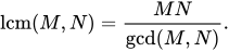
القاسم المشترك الأكبر gcd $(M, N)$ للمتغيرين $M$ و $N$ هو الحد الأحادي ${\textstyle x_{1}^{\min(a_{1},b_{1})}\cdots x_{n}^{\min(a_{n},b_{n})}}$ متجه الأس الذي يمثل أصغر عنصر من عناصر $A$ و $B.$ يتم تعريف المضاعف المشترك الأصغر lcm $(M, N) بشكل مشابه باستخدام$ $القيمة القصوى$ بدلاً من $القيمة الدنيا$ .

يمتلك المرء

\operatorname {lcm} (M,N)={\frac {MN}{\gcd(M,N)}}.

تخفيض

يُعدّ اختزال كثير الحدود بواسطة كثيرات حدود أخرى، وفقًا لترتيب أحادي الحد، أمرًا أساسيًا في نظرية أساس غروبنر. وهو تعميم لكلٍّ من اختزال الصفوف الذي يحدث في عملية الحذف الغاوسي وخطوات القسمة في القسمة الإقليدية لكثيرات الحدود أحادية المتغير . ^{[ 1 ]} وعند إتمامه على أكمل وجه ممكن، يُطلق عليه أحيانًا اسم القسمة متعددة المتغيرات، على الرغم من أن نتيجته ليست محددة بشكل فريد.

يُعدّ اختزال الرصاص حالةً خاصةً من الاختزال، وهو أسهل حسابًا. وهو أساسي لحساب أساس غروبنر، إذ لا يُحتاج إلى الاختزال العام إلا في نهاية حساب أساس غروبنر، وذلك للحصول على أساس غروبنر مُختزل من أساس غير مُختزل.

لنفترض أن ترتيب أحادي الحد مقبول ثابت، والذي تشير إليه كل مقارنة أحادية الحد التي ستحدث في هذا القسم.

تكون كثيرة الحدود $f$ قابلة للاختزال بواسطة كثيرة حدود أخرى $g$ إذا كان الحد الرئيسي $lm(f)$ من مضاعفات $lm(g)$ . وتكون كثيرة الحدود $f$ قابلة للاختزال بواسطة $g$ إذا كان أحد حدودها من مضاعفات $lm$ $(g)$ . (لذا، إذا كانت $f$ قابلة للاختزال بواسطة $g$ ، فهي قابلة للاختزال أيضًا، ولكن قد تكون $f$ قابلة للاختزال دون أن تكون قابلة للاختزال بواسطة g).

لنفترض أن الدالة $f$ قابلة للاختزال بواسطة $g$ ، وليكن $cm$ حدًا من حدود $f$ بحيث يكون الحد الأحادي $m$ مضاعفًا لـ $lm(g)$ . يتكون الاختزال أحادي الخطوة للدالة $f$ بواسطة $g$ من استبدال $f$ بـ

\operatorname {red} _{1}(f,g)=f-{\frac {c}{\operatorname {lc} (g)}}\,{\frac {m}{\operatorname {lm} (g)}}\,g.

تُزيل هذه العملية الحدّ الأحادي $m$ من $f$ دون تغيير الحدود التي يكون فيها الحدّ الأحادي أكبر من $m$ (لترتيب الحدود الأحادية). وعلى وجه الخصوص، ينتج عن اختزال $f$ بخطوة واحدة متعددة حدود تكون جميع حدودها الأحادية أصغر من $lm(f)$ .

بفرض وجود مجموعة منتهية $G$ من كثيرات الحدود، يُقال إن الدالة $f$ قابلة للاختزال أو قابلة للاختزال بالخطوة الأولى بواسطة $G$ إذا كانت قابلة للاختزال أو قابلة للاختزال بالخطوة الأولى، على التوالي، بواسطة عنصر واحد على الأقل $g$ من $G.$ في هذه الحالة، يُعد الاختزال بخطوة واحدة (أو الاختزال بالخطوة الأولى بخطوة واحدة) للدالة $f$ بواسطة $G$ أي اختزال بخطوة واحدة (أو اختزال بالخطوة الأولى بخطوة واحدة) للدالة $f$ بواسطة عنصر من $G.$

يتألف الاختزال (الكامل) (أو اختزال الخطوة الأولى) للدالة $f$ بواسطة $G$ من تكرار عمليات الاختزال أحادية الخطوة (أو اختزال الخطوة الأولى) حتى الحصول على متعددة حدود غير قابلة للاختزال (أو غير قابلة للاختزال) بواسطة $G.$ ويُطلق عليها أحيانًا اسم الشكل الطبيعي للدالة $f$ بواسطة $G.$ وبشكل عام، لا يُعرَّف هذا الشكل تعريفًا فريدًا، لأنه يوجد، في الغالب، عدة عناصر من $G$ يمكن استخدامها لاختزال $f$ ؛ وهذه الخاصية غير الفريدة هي نقطة انطلاق نظرية أساس غروبنر.

يُظهر تعريف الاختزال مباشرةً أنه إذا كانت $h$ شكلًا طبيعيًا لـ $f$ بواسطة $G$ ، فإن المرء لديه

f=h+\sum _{g\in G}q_{g}\,g,

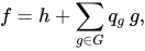
حيث لا يمكن اختزال $h$ بواسطة $G$ و $q_{g}$ هي كثيرات حدود بحيث $\operatorname {lm} (q_{g}\,g)\leq \operatorname {lm} (f).$ في حالة كثيرات الحدود أحادية المتغير، إذا كانت $G$ $تتكون$ من عنصر واحد $g$ ، فإن $h$ هو باقي قسمة $f$ على $g$ باستخدام الإقليد ، و $qg$ هو ناتج القسمة. علاوة على ذلك، فإن خوارزمية القسمة هي عملية اختزال رائدة. لهذا السبب، يستخدم بعض المؤلفين مصطلح القسمة متعددة المتغيرات بدلاً من الاختزال.

عدم تفرد الاختزال

In the example that follows, there are exactly two complete lead-reductions that produce two very different results. The fact that the results are irreducible (not only lead-irreducible) is specific to the example, although this is rather common with such small examples.

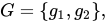
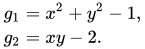
In this two variable example, the monomial ordering that is used is the lexicographic order with $x>y,$ and we consider the reduction of $f=2x^{3}-x^{2}y+y^{3}+3y$ , by $G=\{g_{1},g_{2}\},$ with ${\begin{aligned}g_{1}&=x^{2}+y^{2}-1,\\g_{2}&=xy-2.\end{aligned}}$

For the first reduction step, either the first or the second term of $f$ may be reduced. However, the reduction of a term amounts to removing this term at the cost of adding new lower terms; if it is not the first reducible term that is reduced, it may occur that a further reduction adds a similar term, which must be reduced again. It is therefore always better to reduce first the largest (for the monomial order) reducible term; that is, in particular, to lead-reduce first until getting a lead-irreducible polynomial.

The leading term $2x^{3}$ of $f$ is reducible by $g_{1}$ and not by $g_{2}.$ So the first reduction step consists of multiplying $g_{1}$ by $-2 x$ and adding the result to $f$ : $f\;\xrightarrow {\overset {}{-2xg_{1}}} \;f_{1}=f-2xg_{1}=-x^{2}y-2xy^{2}+2x+y^{3}+3y.$

The leading term $-x^{2}y$ of $f_{1}$ is a multiple of the leading monomials of both $g_{1}$ and $g_{2},$ So, one has two choices for the second reduction step. If one chooses $g_{2},$ one gets a polynomial that can be reduced again by $g_{2}\colon$ $f\;\xrightarrow {\overset {}{-2xg_{1}}} \;f_{1}\;\xrightarrow {xg_{2}} \;-2xy^{2}+y^{3}+3y\;\xrightarrow {2yg_{2}} \;f_{2}=y^{3}-y.$ No further reduction is possible, so $f_{2}$ is a complete reduction of $f$ .

One gets a different result with the other choice for the second step: $f\;\xrightarrow {\overset {}{-2xg_{1}}} \;f_{1}\;\xrightarrow {yg_{1}} \;-2xy^{2}+2x+2y^{3}+2y\;\xrightarrow {2yg_{2}} \;f_{3}=2x+2y^{3}-2y.$ Again, the result $f_{3}$ is irreducible, although only lead reductions were done.

In summary, the complete reduction of $f$ can result in either $f_{2}=y^{3}-y$ or $f_{3}=2x+2y^{3}-2y.$

It is for dealing with the problems set by this non-uniqueness that Buchberger introduced Gröbner bases and $S$ -polynomials. Intuitively, $0=f-f$ may be reduced to $f_{2}-f_{3}.$ This implies that $f_{2}-f_{3}$ belongs to the ideal generated by $G$ . So, this ideal is not changed by adding $f_{3}-f_{2}$ to $G$ , and this allows more reductions. In particular, $f_{3}$ can be reduced to $f_{2}$ by $f_{3}-f_{2}$ and this restores the uniqueness of the reduced form.

Here Buchberger's algorithm for Gröbner bases would begin by adding to $G$ the polynomial

g_{3}=yg_{1}-xg_{2}=2x+y^{3}-y.

This polynomial, called $S$ -polynomial by Buchberger, is the difference of the one-step reductions of the least common multiple $x^{2}y$ of the leading monomials of $g_{1}$ and $g_{2}$ , by $g_{2}$ and $g_{1}$ respectively:

g_{3}=\left(x^{2}y-{\frac {x^{2}y}{\mathrm {lt} (g_{2})}}g_{2}\right)-\left(x^{2}y-{\frac {x^{2}y}{\mathrm {lt} (g_{1})}}g_{1}\right)={\frac {x^{2}y}{\mathrm {lt} (g_{1})}}g_{1}-{\frac {x^{2}y}{\mathrm {lt} (g_{2})}}g_{2}

.

In this example, one has $g_{3}=f_{3}-f_{2}.$ This does not complete Buchberger's algorithm, as $xy$ gives different results, when reduced by $g_{2}$ or $g_{3}.$

S-polynomial

Given monomial ordering, the S-polynomial or critical pair of two polynomials $f$ and $g$ is the polynomial

S(f,g)=\operatorname {red} _{1}(\mathrm {lcm} ,g)-\operatorname {red} _{1}(\mathrm {lcm} ,f)

;

where $lcm$ denotes the least common multiple of the leading monomials of $f$ and $g$ . Using the definition of $\operatorname {red} _{1}$ , this translates to:

{\begin{aligned}S(f,g)&=\left(\mathrm {lcm} -{\frac {1}{\operatorname {lc} (g)}}\,{\frac {\mathrm {lcm} }{\operatorname {lm} (g)}}\,g\right)-\left(\mathrm {lcm} -{\frac {1}{\operatorname {lc} (f)}}\,{\frac {\mathrm {lcm} }{\operatorname {lm} (f)}}\,f\right)\\&={\frac {1}{\operatorname {lc} (f)}}\,{\frac {\mathrm {lcm} }{\operatorname {lm} (f)}}\,f-{\frac {1}{\operatorname {lc} (g)}}\,{\frac {\mathrm {lcm} }{\operatorname {lm} (g)}}\,g\\\end{aligned}}.

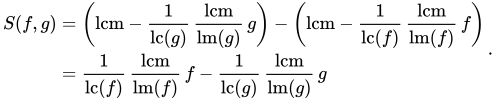
Using the property that relates the $lcm$ and the $gcd$ , the S-polynomial can also be written as:

S(f,g)={\frac {1}{\operatorname {lc} (f)}}\,{\frac {\operatorname {lm} (g)}{\mathrm {gcd} }}\,f-{\frac {1}{\operatorname {lc} (g)}}\,{\frac {\operatorname {lm} (f)}{\mathrm {gcd} }}\,g;

where $gcd$ denotes the greatest common divisor of the leading monomials of $f$ and $g$ .

As the monomials that are reducible by both $f$ and $g$ are exactly the multiples of $lcm$ , one can deal with all cases of non-uniqueness of the reduction by considering only the S-polynomials. This is a fundamental fact for Gröbner basis theory and all algorithms for computing them.

For avoiding fractions when dealing with polynomials with integer coefficients, the S polynomial is often defined as

S(f,g)=\operatorname {lc} (g)\,{\frac {\operatorname {lm} (g)}{\mathrm {gcd} }}\,f-\operatorname {lc} (f)\,{\frac {\operatorname {lm} (f)}{\mathrm {gcd} }}\,g;

This does not change anything to the theory since the two polynomials are associates.

Definition

Let $R=F[x_{1},\ldots ,x_{n}]$ be a polynomial ring over a field $F$ . In this section, we suppose that an admissible monomial ordering has been fixed.

Let $G$ be a finite set of polynomials in $R$ that generates an ideal $I$ . The set $G$ is a Gröbner basis (with respect to the monomial ordering), or, more precisely, a Gröbner basis of $I$ if

the ideal generated by the leading monomials of the polynomials in $I$ equals the ideal generated by the leading monomials of $G$ ,

or, equivalently,

the leading monomial of every polynomial in $I$ is a multiple of the leading monomial of some polynomial in $G$ .

There are many characterizing properties, which can each be taken as an equivalent definition of Gröbner bases. For conciseness, in the following list, the notation "one-word/another word" means that one can take either "one-word" or "another word" for having two different characterizations of Gröbner bases. All the following assertions are characterizations of Gröbner bases:

a polynomial $f$ is in $I$ , if and only if some/every complete lead-reduction/reduction of $f$ by $G$ produces the zero polynomial;
لكل متعدد حدود $S$ $من$ عناصر $G$ ، ينتج عن بعض/كل اختزال كامل للعنصر $s$ بواسطة $G$ الصفر؛
جميع عمليات الاختزال الكاملة لعنصر من $R$ تنتج نفس النتيجة؛
تشكل أحاديات الحدود غير القابلة للاختزال بواسطة $G$ أساسًا للفضاء المتجهي $F$ $R/I.$

بإضافة التعريف المذكور أعلاه، يُقدّم هذا 12 وصفًا لقواعد غروبنر. إنّ كثرة هذه الأوصاف تجعل قواعد غروبنر مفيدة للغاية. على سبيل المثال، يُقدّم الشرط 3 خوارزمية لاختبار الانتماء المثالي ؛ ويُقدّم الشرط 4 خوارزمية لاختبار ما إذا كانت مجموعة من كثيرات الحدود تُشكّل قاعدة غروبنر، ويُشكّل أساس خوارزمية بوخبيرغر لحساب قواعد غروبنر؛ ويسمح الشرطان 5 و6 بالحساب في $R/I$ بطريقة تشبه إلى حد كبير الحساب النمطي .

وجود

لكل ترتيب أحادي مقبول ولكل مجموعة منتهية $G$ من كثيرات الحدود، توجد قاعدة غروبنر تحتوي على $G$ وتولد نفس المثالي. علاوة على ذلك، يمكن حساب قاعدة غروبنر هذه باستخدام خوارزمية بوخبيرغر .

تستخدم هذه الخوارزمية الشرط 4، وتسير تقريبًا على النحو التالي: لأي عنصرين من $G$ ، احسب الاختزال الكامل بواسطة $G لكثير الحدود$ S الخاص بهما ، وأضف النتيجة إلى $G$ إذا لم تكن صفرًا؛ كرر هذه العملية مع تضمين العناصر الجديدة من $G$ حتى، في النهاية، تنتج جميع عمليات الاختزال صفرًا.

تنتهي الخوارزمية دائمًا إما بسبب مبرهنة ديكسون أو لأن حلقات كثيرات الحدود نوثرية ( مبرهنة هيلبرت للأساس ). يضمن الشرط 4 أن تكون النتيجة أساس غروبنر، وتضمن تعريفات كثيرات الحدود S والاختزال عدم تغيير المثالي المُوَلَّد.

الطريقة المذكورة أعلاه هي خوارزمية لحساب قواعد غروبنر، إلا أنها غير فعّالة للغاية. وقد طُرحت العديد من التحسينات على خوارزمية بوخبيرغر الأصلية، بالإضافة إلى خوارزميات أخرى، وتم تطبيقها، مما أدى إلى تحسين الكفاءة بشكل ملحوظ. انظر قسم الخوارزميات والتطبيقات أدناه.

قواعد جروبنر المخفضة

أساس غروبنر هوتكون مجموعة غروبنر صغرى إذا كانت جميع الحدود الرئيسية لعناصرها غير قابلة للاختزال بواسطة العناصر الأخرى للمجموعة الأساسية. بفرض وجود مجموعة أساسية غروبنر لمثالي $I$ ، نحصل على مجموعة أساسية غروبنر صغرى لـ $I$ بإزالة كثيرات الحدود التي تكون حدودها الرئيسية من مضاعفات الحد الرئيسي لعنصر آخر من مجموعة غروبنر. مع ذلك، إذا كان لكثيرتي حدود في المجموعة الأساسية نفس الحد الرئيسي، فيجب إزالة إحداهما فقط. لذا، تحتوي كل مجموعة أساسية غروبنر على مجموعة أساسية غروبنر صغرى كمجموعة جزئية.

جميع قواعد غروبنر الدنيا لمثال معين (لترتيب أحادي ثابت) لها نفس عدد العناصر، ونفس الأحاديات الرائدة، وقواعد غروبنر غير الدنيا لها عناصر أكثر من القواعد الدنيا.

أساس غروبنر هوتُختزل قاعدة غروبنر إذا كانت كل كثيرة حدود فيها غير قابلة للاختزال بواسطة العناصر الأخرى للقاعدة، وكان $1.$ لذا، فإن كل قاعدة غروبنر مُختزلة هي قاعدة دنيا، ولكن قاعدة غروبنر الدنيا ليست بالضرورة مُختزلة.

بالنظر إلى أساس غروبنر لمثالي $I$ ، يمكن الحصول على أساس غروبنر مختزل لـ $I$ عن طريق إزالة كثيرات الحدود التي يمكن اختزالها بواسطة عناصر أخرى من الأساس (للحصول على أساس أدنى)؛ ثم استبدال كل عنصر من الأساس بنتيجة الاختزال الكامل بواسطة العناصر الأخرى من الأساس؛ وأخيرًا، عن طريق قسمة كل عنصر من الأساس على معامله الرئيسي.

جميع قواعد غروبنر المختزلة لمثالي (لترتيب أحادي ثابت) متساوية. ويترتب على ذلك أن مثاليين متساويان إذا وفقط إذا كان لهما نفس قاعدة غروبنر المختزلة.

أحيانًا، تُعرَّف قواعد غروبنر المختزلة دون اشتراط المعاملات الرئيسية. في هذه الحالة، تكون خاصية تفرد قواعد غروبنر المختزلة صحيحة فقط حتى ضرب كثيرات الحدود بثابت غير صفري.

عند التعامل مع كثيرات الحدود على الحقل $\mathbb {Q}$ من بين الأعداد النسبية ، من المفيد التعامل فقط مع كثيرات الحدود ذات المعاملات الصحيحة. في هذه الحالة، يمكن استبدال شرط المعاملات الرئيسية في تعريف الأساس المختزل بشرط أن تكون جميع عناصر الأساس كثيرات حدود أولية ذات معاملات صحيحة، ومعاملات رئيسية موجبة. وهذا يُعيد تفرد الأسس المختزلة.

حالات خاصة

لكل ترتيب أحادي الحد، فإن المجموعة الفارغة من كثيرات الحدود هي أساس غروبنر الوحيد للمثال الصفري .

لكل ترتيب أحادي الحد، تُشكّل مجموعة كثيرات الحدود التي تحتوي على ثابت غير صفري أساس غروبنر للمثالي الواحد (حلقة كثيرات الحدود بأكملها). وبالعكس، يحتوي كل أساس غروبنر للمثالي الواحد على ثابت غير صفري. ويتكون أساس غروبنر المُختزل للمثالي الواحد من كثيرة الحدود المفردة $1$ .

In the case of polynomials in a single variable, there is a unique admissible monomial ordering, the ordering by the degree. The minimal Gröbner bases are the singletons consisting of a single polynomial. The reduced Gröbner bases are the monic polynomials.

Example and counterexample

{\displaystyle f} — The zeroes of $f$ form the red parabola; the zeroes of $g$ form the three blue vertical lines. Their intersection consists of three points.

Let $R=\mathbb {Q} [x,y]$ be the ring of bivariate polynomials with rational coefficients and consider the ideal $I=\langle f,g\rangle$ generated by the polynomials

f=x^{2}-y

,

g=x^{3}-x

.

By reducing $g$ by $f$ , one obtains a new polynomial $k$ such that ${\displaystyle I=\langle f,k\rangle$

k=g-xf=xy-x.

None of $f$ and $k$ is reducible by the other, but $xk$ is reducible by $f$ , which gives another polynomial in $I$ :

h=xk-(y-1)f=y^{2}-y.

Under lexicographic ordering with $x>y$ we have

\mathrm {lt} (f)=x^{2}

\mathrm {lt} (k)=xy

\mathrm {lt} (h)=y^{2}

As $f, k$ and $h$ belong to $I$ , and none of them is reducible by the others, none of $\{f,k\},$ $\{f,h\},$ and $\{h,k\}$ is a Gröbner basis of $I$ .

On the other hand, ${f, k, h}$ is a Gröbner basis of $I$ , since the S-polynomials

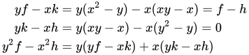
{\begin{aligned}yf-xk&=y(x^{2}-y)-x(xy-x)=f-h\\yk-xh&=y(xy-x)-x(y^{2}-y)=0\\y^{2}f-x^{2}h&=y(yf-xk)+x(yk-xh)\end{aligned}}

can be reduced to zero by $f, k$ and $h$ .

The method that has been used here for finding $h$ and $k$ , and proving that ${f, k, h}$ is a Gröbner basis is a direct application of Buchberger's algorithm. So, it can be applied mechanically to any similar example, although, in general, there are many polynomials and S-polynomials to consider, and the computation is generally too large for being done without a computer.

Properties and applications of Gröbner bases

Unless explicitly stated, all the results that follow^[3] are true for any monomial ordering (see that article for the definitions of the different orders that are mentioned below).

It is a common misconception that the lexicographical order is needed for some of these results. On the contrary, the lexicographical order is, almost always, the most difficult to compute, and using it makes impractical many computations that are relatively easy with graded reverse lexicographic order (grevlex), or, when elimination is needed, the elimination order (lexdeg) which restricts to grevlex on each block of variables.

Equality of ideals

تكون قواعد غروبنر المختزلة فريدة لأي مثالي معين وأي ترتيب أحادي الحد. وبالتالي، يكون مثاليان متساويين إذا وفقط إذا كان لهما نفس قاعدة غروبنر (المختزلة) (عادةً ما ينتج برنامج قاعدة غروبنر دائمًا قواعد غروبنر مختزلة).

العضوية وإدماج المُثُل

يؤدي اختزال متعددة الحدود f باستخدام أساس غروبنر G للمثالي $I$ إلى صفر إذا وفقط إذا كانت f تنتمي إلى $I.$ وهذا يسمح باختبار انتماء عنصر ما إلى المثالي. وتتمثل طريقة أخرى في التحقق من أن أساس غروبنر لـ G $\cup {f}$ يساوي G.

لاختبار ما إذا كان المثالي $I$ المُوَلَّد بواسطة $f 1, ..., f k$ مُحتوى في المثالي $J$ ، يكفي اختبار أن كل $f I$ ينتمي إلى $J.$ ويمكن أيضًا اختبار تساوي قواعد غروبنر المُختزلة لـ $J$ و $J \cup {f 1, ..., f k}$ .

حلول نظام المعادلات الجبرية

يمكن اعتبار أي مجموعة من كثيرات الحدود نظامًا من المعادلات متعددة الحدود بمساواة كثيرات الحدود بالصفر. تعتمد مجموعة حلول هذا النظام فقط على المثالي المُوَلَّد، وبالتالي لا تتغير عند استبدال مجموعة التوليد المعطاة بقاعدة غروبنر، لأي ترتيب، للمثالي المُوَلَّد. يُسمى هذا الحل، بإحداثياته في حقل مغلق جبريًا يحتوي على معاملات كثيرات الحدود، صفرًا للمثالي . في الحالة المعتادة للمعاملات النسبية ، يُختار هذا الحقل المغلق جبريًا كحقل عقدي .

لا يحتوي المثالي على أي صفر (نظام المعادلات غير متسق ) إذا وفقط إذا كان 1 ينتمي إلى المثالي (هذه هي نظرية هيلبرت للأصفار )، أو بشكل مكافئ، إذا كانت قاعدة جروبنر الخاصة به (لأي ترتيب أحادي الحد) تحتوي على 1، أو أيضًا، إذا كانت قاعدة جروبنر المختزلة المقابلة هي [1].

إذا كانت لدينا قاعدة غروبنر G للمثالي I ، فإن هذه القاعدة تحتوي على عدد محدود من الأصفار، إذا وفقط إذا احتوت G ، لكل متغير x ، على متعددة حدود يكون حدها الرئيسي قوةً لـ x (دون ظهور أي متغير آخر في الحد الرئيسي). في هذه الحالة، يكون عدد الأصفار، مع مراعاة التكرار، مساويًا لعدد الحدود التي ليست مضاعفات لأي حد رئيسي في G. يُسمى هذا العدد درجة المثالي.

عندما يكون عدد الأصفار محدودًا، توفر قاعدة غروبنر لترتيب أحاديات الحدود المعجمي، نظريًا، حلًا: الإحداثي الأول للحل هو جذر القاسم المشترك الأكبر لكثيرات الحدود في القاعدة التي تعتمد فقط على المتغير الأول. بعد استبدال هذا الجذر في القاعدة، يكون الإحداثي الثاني لهذا الحل هو جذر القاسم المشترك الأكبر لكثيرات الحدود الناتجة التي تعتمد فقط على المتغير الثاني، وهكذا. عملية الحل هذه نظرية فقط، لأنها تتضمن حساب القاسم المشترك الأكبر وإيجاد جذور كثيرات الحدود ذات المعاملات التقريبية، وهو أمر غير عملي بسبب عدم الاستقرار العددي. لذلك، طُوّرت طرق أخرى لحل أنظمة كثيرات الحدود باستخدام قواعد غروبنر (انظر نظام معادلات كثيرات الحدود لمزيد من التفاصيل).

الأبعاد والدرجات ومتسلسلات هيلبرت

بُعد المثالي I في حلقة كثيرات الحدود R هو بُعد كرول للحلقة R / I ، وهو يساوي بُعد المجموعة الجبرية لأصفار I. كما يساوي عدد المستويات الفائقة في الوضع العام اللازمة للتقاطع مع المجموعة الجبرية، وهو عدد محدود من النقاط. درجة المثالي ومجموعته الجبرية المرتبطة به هي عدد نقاط هذا التقاطع المحدود، مع مراعاة التعددية. على وجه الخصوص، درجة السطح الفائق تساوي درجة كثير الحدود التعريفي الخاص به.

يعتمد البُعد فقط على مجموعة أحاديات الحدود الرئيسية لقاعدة غروبنر للمثالي لأي ترتيب أحادي الحدود. وينطبق الأمر نفسه على ترتيبات أحاديات الحدود من الدرجة وترتيبات أحاديات الحدود المتوافقة مع الدرجة؛ يكون ترتيب أحادي الحدود متوافقًا مع الدرجة إذا كان أصغر بالنسبة للدرجة يعني أصغر بالنسبة لترتيب أحادي الحدود.

The dimension is the maximal size of a subset S of the variables such that there is no leading monomial depending only on the variables in S. Thus, if the ideal has dimension 0, then for each variable x there is a leading monomial in the Gröbner basis that is a power of $x$ .

Both dimension and degree may be deduced from the Hilbert series of the ideal, which is the series ${\textstyle \sum _{i=0}^{\infty }d_{i}t^{i}}$ , where $d_{i}$ is the number of monomials of degree i that are not multiple of any leading monomial in the Gröbner basis.^[4] The Hilbert series may be summed into a rational fraction

\sum _{i=0}^{\infty }d_{i}t^{i}={\frac {P(t)}{(1-t)^{d}}},

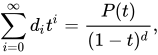
where d is the dimension of the ideal and $P(t)$ is a polynomial. The number $P(1)$ is the degree of the algebraic set defined by the ideal, in the case of a homogeneous ideal or a monomial ordering compatible with the degree; that is, to compare two monomials, one compares their total degrees first.

The dimension does not depend on the choice of a monomial ordering, although the Hilbert series and the polynomial $P(t)$ may change with changes of the monomial ordering. However, for homogeneous ideals or monomial orderings compatible with the degree, the Hilbert series and the polynomial $P(t)$ do not depend on the choice of monomial ordering.^[5]

Most computer algebra systems that provide functions to compute Gröbner bases provide also functions for computing the Hilbert series, and thus also the dimension and the degree.

Elimination

The computation of Gröbner bases for an elimination monomial ordering allows computational elimination theory. This is based on the following theorem.

Consider a polynomial ring $K[x_{1},\ldots ,x_{n},y_{1},\ldots ,y_{m}]=K[X,Y],$ in which the variables are split into two subsets X and Y. Let us also choose an elimination monomial ordering "eliminating" X, that is a monomial ordering for which two monomials are compared by comparing first the X-parts, and, in case of equality only, considering the Y-parts. This implies that a monomial containing an X-variable is greater than every monomial independent of X. If G is a Gröbner basis of an ideal I for this monomial ordering, then $G\cap K[Y]$ is a Gröbner basis of $I\cap K[Y]$ (this ideal is often called the elimination ideal). Moreover, $G\cap K[Y]$ consists exactly of the polynomials of $G$ whose leading terms belong to $K [Y]$ (this makes the computation of $G\cap K[Y]$ very easy, as only the leading monomials need to be checked).

This elimination property has many applications, some described in the next sections.

Another application, in algebraic geometry, is that elimination realizes the geometric operation of projection of an affine algebraic set into a subspace of the ambient space: with above notation, the (Zariski closure of) the projection of the algebraic set defined by the ideal I into the Y-subspace is defined by the ideal $I\cap K[Y].$

The lexicographical ordering such that $x_{1}>\cdots >x_{n}$ is an elimination ordering for every partition $\{x_{1},\ldots ,x_{k}\},\{x_{k+1},\ldots ,x_{n}\}.$ Thus a Gröbner basis for this ordering carries much more information than usually necessary. This may explain why Gröbner bases for the lexicographical ordering are usually the most difficult to compute.

Intersecting ideals

If $I$ and $J$ are two ideals generated respectively by {f₁, ..., f_m} and {g₁, ..., g_k}, then a single Gröbner basis computation produces a Gröbner basis of their intersection $I \cap J$ . For this, one introduces a new indeterminate t, and one uses an elimination ordering such that the first block contains only t and the other block contains all the other variables (this means that a monomial containing t is greater than every monomial that does not contain t). With this monomial ordering, a Gröbner basis of $I \cap J$ consists in the polynomials that do not contain t, in the Gröbner basis of the ideal

K=\langle tf_{1},\ldots ,tf_{m},(1-t)g_{1},\ldots ,(1-t)g_{k}\rangle .

In other words, $I \cap J$ is obtained by eliminatingt in K. This may be proven by observing that the ideal K consists of the polynomials $(a-b)t+b$ such that $a\in I$ and $b\in J$ . Such a polynomial is independent of t if and only if $a = b$ , which means that $b\in I\cap J.$

Implicitization of a rational curve

A rational curve is an algebraic curve that has a set of parametric equations of the form

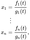
{\begin{aligned}x_{1}&={\frac {f_{1}(t)}{g_{1}(t)}}\\&\;\;\vdots \\x_{n}&={\frac {f_{n}(t)}{g_{n}(t)}},\end{aligned}}

where $f_{i}(t)$ and $g_{i}(t)$ are univariate polynomials for 1 ≤ i ≤ n. One may (and will) suppose that $f_{i}(t)$ and $g_{i}(t)$ are coprime (they have no non-constant common factors).

Implicitization consists in computing the implicit equations of such a curve. In case of n = 2, that is for plane curves, this may be computed with the resultant. The implicit equation is the following resultant:

{\text{Res}}_{t}(g_{1}x_{1}-f_{1},g_{2}x_{2}-f_{2}).

Elimination with Gröbner bases allows to implicitize for any value of n, simply by eliminating t in the ideal $\langle g_{1}x_{1}-f_{1},\ldots ,g_{n}x_{n}-f_{n}\rangle .$ If n = 2, the result is the same as with the resultant, if the map $t\mapsto (x_{1},x_{2})$ is injective for almost every t. In the other case, the resultant is a power of the result of the elimination.

Saturation

When modeling a problem by polynomial equations, it is often assumed that some quantities are non-zero, so as to avoid degenerate cases. For example, when dealing with triangles, many properties become false if the triangle degenerates to a line segment, i.e. the length of one side is equal to the sum of the lengths of the other sides. In such situations, one cannot deduce relevant information from the polynomial system unless the degenerate solutions are ignored. More precisely, the system of equations defines an algebraic set which may have several irreducible components, and one must remove the components on which the degeneracy conditions are everywhere zero.

This is done by saturating the equations by the degeneracy conditions, which may be done via the elimination property of Gröbner bases.

Definition of the saturation

The localization of a ring consists in adjoining to it the formal inverses of some elements. This section concerns only the case of a single element, or equivalently a finite number of elements (adjoining the inverses of several elements is equivalent to adjoining the inverse of their product). The localization of a ring R by an element f is the ring $R_{f}=R[t]/(1-ft),$ where t is a new indeterminate representing the inverse of f. The localization of an ideal $I$ of R is the ideal $I_{f}=R_{f}I$ of $R_{f}.$ When R is a polynomial ring, computing in $R_{f}$ is not efficient because of the need to manage the denominators. Therefore, localization is usually replaced by the operation of saturation.

The saturation with respect to f of an ideal $I$ in R is the inverse image of $R_{f}I$ under the canonical map from R to $R_{f}.$ It is the ideal $I:f^{\infty }=\{g\in R\mid (\exists k\in \mathbb {N} )f^{k}g\in I\}$ consisting in all elements of R whose product with some power of f belongs to $I$ .

If $J$ is the ideal generated by $I$ and 1−ft in R[t], then $I:f^{\infty }=J\cap R.$ It follows that, if R is a polynomial ring, a Gröbner basis computation eliminating t produces a Gröbner basis of the saturation of an ideal by a polynomial.

The important property of the saturation, which ensures that it removes from the algebraic set defined by the ideal $I$ the irreducible components on which the polynomial f is zero, is the following: The primary decomposition of $I:f^{\infty }$ consists of the components of the primary decomposition of I that do not contain any power of f.

Computation of the saturation

A Gröbner basis of the saturation by f of a polynomial ideal generated by a finite set of polynomials F, may be obtained by eliminating t in $F\cup \{1-tf\},$ that is by keeping the polynomials independent of t in the Gröbner basis of $F\cup \{1-tf\}$ for an elimination ordering eliminating t.

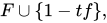
Instead of using F, one may also start from a Gröbner basis of F. Which method is most efficient depends on the problem. However, if the saturation does not remove any component, that is if the ideal is equal to its saturated ideal, computing first the Gröbner basis of F is usually faster. On the other hand, if the saturation removes some components, the direct computation may be dramatically faster.

If one wants to saturate with respect to several polynomials $f_{1},\ldots ,f_{k}$ or with respect to a single polynomial which is a product $f=f_{1}\cdots f_{k},$ there are three ways to proceed which give the same result but may have very different computation times (it depends on the problem which is the most efficient).

Saturating by $f=f_{1}\cdots f_{k}$ in a single Gröbner basis computation.
Saturating by $f_{1},$ then saturating the result by $f_{2},$ and so on.
Adding to F or to its Gröbner basis the polynomials $1-t_{1}f_{1},\ldots ,1-t_{k}f_{k},$ and eliminating the $t_{i}$ in a single Gröbner basis computation.

Effective Nullstellensatz

Hilbert's Nullstellensatz has two versions. The first one asserts that a set of polynomials has no common zeros over an algebraic closure of the field of the coefficients, if and only if 1 belongs to the generated ideal. This is easily tested with a Gröbner basis computation, because 1 belongs to an ideal if and only if 1 belongs to the Gröbner basis of the ideal, for any monomial ordering.

The second version asserts that the set of common zeros (in an algebraic closure of the field of the coefficients) of an ideal is contained in the hypersurface of the zeros of a polynomial f, if and only if a power of f belongs to the ideal. This may be tested by saturating the ideal by f; in fact, a power of f belongs to the ideal if and only if the saturation by f provides a Gröbner basis containing 1.

Implicitization in higher dimension

By definition, an affine rational variety of dimension k may be described by parametric equations of the form

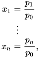
{\begin{aligned}x_{1}&={\frac {p_{1}}{p_{0}}}\\&\;\;\vdots \\x_{n}&={\frac {p_{n}}{p_{0}}},\end{aligned}}

where $p_{0},\ldots ,p_{n}$ are n+1 polynomials in the k variables (parameters of the parameterization) $t_{1},\ldots ,t_{k}.$ Thus the parameters $t_{1},\ldots ,t_{k}$ and the coordinates $x_{1},\ldots ,x_{n}$ of the points of the variety are zeros of the ideal

I=\left\langle p_{0}x_{1}-p_{1},\ldots ,p_{0}x_{n}-p_{n}\right\rangle .

One could guess that it suffices to eliminate the parameters to obtain the implicit equations of the variety, as it has been done in the case of curves. Unfortunately this is not always the case. If the $p_{i}$ have a common zero (sometimes called base point), every irreducible component of the non-empty algebraic set defined by the $p_{i}$ is an irreducible component of the algebraic set defined by I. It follows that, in this case, the direct elimination of the $t_{i}$ provides an empty set of polynomials.

Therefore, if k>1, two Gröbner basis computations are needed to implicitize:

Saturate $I$ by $p_{0}$ to get a Gröbner basis $G$
Eliminate the $t_{i}$ from $G$ to get a Gröbner basis of the ideal (of the implicit equations) of the variety.

Algorithms and implementations

Buchberger's algorithm is the oldest algorithm for computing Gröbner bases. It was devised by Bruno Buchberger together with the Gröbner basis theory. It is straightforward to implement, but it appeared soon that raw implementations can solve only trivial problems. The main issues are the following ones:

Even when the resulting Gröbner basis is small, the intermediate polynomials can be huge. It results that most of the computing time may be spent in memory management. So, specialized memory management algorithms may be a fundamental part of an efficient implementation.
The integers occurring during a computation may be sufficiently large for making fast multiplication algorithms and multimodular arithmetic useful. For this reason, most optimized implementations use the GMP library. Also, modular arithmetic, Chinese remainder theorem and Hensel lifting are used in optimized implementations
The choice of the S-polynomials to reduce and of the polynomials used for reducing them is devoted to heuristics. As in many computational problems, heuristics cannot detect most hidden simplifications, and if heuristic choices are avoided, one may get a dramatic improvement of the algorithm efficiency.
In most cases most S-polynomials that are computed are reduced to zero; that is, most computing time is spent to compute zero.
The monomial ordering that is most often needed for the applications (pure lexicographic) is not the ordering that leads to the easiest computation, generally the ordering degrevlex.

For solving 3. many improvements, variants and heuristics have been proposed before the introduction of F4 and F5 algorithms by Jean-Charles Faugère. As these algorithms are designed for integer coefficients or with coefficients in the integers modulo a prime number, Buchberger's algorithm remains useful for more general coefficients.

Roughly speaking, F4 algorithm solves 3. by replacing many S-polynomial reductions by the row reduction of a single large matrix for which advanced methods of linear algebra can be used. This solves partially issue 4., as reductions to zero in Buchberger's algorithm correspond to relations between rows of the matrix to be reduced, and the zero rows of the reduced matrix correspond to a basis of the vector space of these relations.

تُحسّن خوارزمية F5 خوارزمية F4 من خلال إدخال معيار يسمح بتقليل حجم المصفوفات المراد اختزالها. هذا المعيار مثالي تقريبًا، نظرًا لأن المصفوفات المراد اختزالها تكون كاملة الرتبة في الحالات المنتظمة بدرجة كافية (خاصةً عندما تُشكّل كثيرات الحدود المُدخلة متتالية منتظمة ). يُعدّ ضبط خوارزمية F5 للاستخدام العام أمرًا صعبًا، لأن أداءها يعتمد على ترتيب كثيرات الحدود المُدخلة والتوازن بين زيادة درجة كثيرة الحدود العاملة وعدد كثيرات الحدود المُدخلة التي يتم أخذها في الاعتبار. حتى الآن (2022)، لا يوجد تطبيق موزّع أكثر كفاءة بشكل ملحوظ من خوارزمية F4، ولكن، على الأعداد الصحيحة المعيارية، استُخدمت خوارزمية F5 بنجاح في العديد من تحديات التشفير ؛ على سبيل المثال، لفكّ خوارزمية HFE .

تم حل المشكلة رقم 5 باكتشاف خوارزميات تحويل الأساس التي تبدأ من أساس غروبنر لترتيب أحادي الحد لحساب أساس غروبنر لترتيب أحادي الحد آخر. خوارزمية FGLM هي إحدى خوارزميات تحويل الأساس هذه، وهي تعمل فقط في الحالة الصفرية الأبعاد (حيث يكون لكثيرات الحدود عدد محدود من الأصفار المشتركة المركبة)، ولها تعقيد متعدد الحدود بالنسبة لعدد الأصفار المشتركة. أما خوارزمية تحويل الأساس التي تعمل في الحالة العامة فهي خوارزمية مسار غروبنر . ^{[ 6 ]} في شكلها الأصلي، قد تكون خوارزمية FGLM هي الخطوة الحاسمة لحل أنظمة المعادلات متعددة الحدود، لأن خوارزمية FGLM لا تأخذ في الحسبان تباعد المصفوفات المعنية . وقد تم تدارك هذا الأمر من خلال تقديم خوارزميات FGLM المتباعدة . ^{[ 7 ]}

تتضمن معظم أنظمة الجبر الحاسوبية العامة تطبيقات لخوارزمية واحدة أو أكثر لقواعد غروبنر، وغالبًا ما تكون هذه التطبيقات مُدمجة في وظائف أخرى، مثل حل أنظمة المعادلات متعددة الحدود أو تبسيط الدوال المثلثية ؛ وهذا ينطبق، على سبيل المثال، على CoCoA و GAP و Macaulay 2 و Magma و Maple و Mathematica و SINGULAR و SageMath و SymPy . وعند توفر F4، يكون عادةً أكثر كفاءة من خوارزمية بوخبيرغر. لا تُوثَّق دائمًا تقنيات التنفيذ والمتغيرات الخوارزمية، على الرغم من أنها قد تُحدث فرقًا كبيرًا في الكفاءة.

تتضمن مكتبة Msolve تطبيقات لخوارزميتي F4 و(sparse)-FGLM . ^{[ 8 ]} بالإضافة إلى خوارزميات Gröbner، تحتوي Msolve على خوارزميات سريعة لعزل الجذور الحقيقية ، وتجمع كل هذه الوظائف في خوارزمية لإيجاد الحلول الحقيقية لأنظمة المعادلات متعددة الحدود ، والتي تتفوق بشكل ملحوظ على البرامج الأخرى المخصصة لهذه المسألة (Maple وMagma). ^{[ 8 ]} تتوفر Msolve على GitHub ، وتتكامل مع Julia وMaple وSageMath؛ مما يعني إمكانية استخدامها مباشرةً من داخل هذه البيئات البرمجية.

تعقيد

$يتم$ تقييم تعقيد حسابات أساس جروبنر عادةً من حيث عدد المتغيرات $n$ والدرجة القصوى d لكثيرات الحدود المدخلة.

في أسوأ الأحوال، يكون المعيار الرئيسي للتعقيد هو الدرجة القصوى لعناصر أساس غروبنر المختزل الناتج. وبشكل أدق، إذا كان أساس غروبنر يحتوي على عنصر ذي درجة كبيرة $D$ ، فقد يحتوي هذا العنصر على $\Omega (D^{n})$ الحدود غير الصفرية التي يتطلب حسابها وقتًا قدره $\Omega (D^{n})>D^{\Omega (n)}.$ من ناحية أخرى، إذا كانت جميع كثيرات الحدود في أساس غروبنر المختزل لمثالي متجانس لها درجة لا تتجاوز $D$ ، فيمكن حساب أساس غروبنر بواسطة الجبر الخطي على فضاء المتجهات لكثيرات الحدود ذات الدرجة الأقل من $2D ،$ والذي له بُعد $O(D^{n}).$ ^{[ 1 ]} إذن، فإن تعقيد هذه العملية الحسابية هو $O(D^{n})^{O(1)}=D^{O(n)}.$

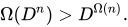
إن تعقيد أسوأ حالة لحساب أساس غروبنر هو أسّي مضاعف بالنسبة إلى $n$ . وبشكل أدق، فإن التعقيد محدود من الأعلى بكثير حدودي في ${\textstyle d^{2^{n}}.}$ باستخدام رمز o الصغير ، فإنها بالتالي محدودة بـ ${\textstyle d^{2^{n+o(n)}}.}$ من ناحية أخرى، تم تقديم أمثلة على قواعد غروبنر المختزلة التي تحتوي على كثيرات حدود من الدرجة ${\textstyle d^{2^{\Omega (n)}},}$ أو تحتوي على ${\textstyle d^{2^{\Omega (n)}}}$ العناصر. بما أن كل خوارزمية لحساب أساس جروبنر يجب أن تكتب نتيجتها، فإن هذا يوفر حدًا أدنى للتعقيد.

أساس غروبنر هو EXPSPACE-كامل . ^{[ 9 ]}

التعميمات

تم تعميم مفهوم وخوارزميات قواعد غروبنر لتشمل الوحدات الفرعية للوحدات الحرة على حلقة متعددة الحدود. في الواقع، إذا كانت $L$ وحدة حرة على حلقة $R$ ، فيمكن حينها النظر في المجموع المباشر. $R\oplus L$ يمكن تعريف هذه الحلقة بأنها حلقة من خلال تعريف حاصل ضرب عنصرين من $L$ بأنه يساوي $صفرًا$ . ويمكن تحديد هذه الحلقة مع $R[e_{1},\ldots ,e_{l}]/\left\langle \{e_{i}e_{j}|1\leq i\leq j\leq l\}\right\rangle$ ، أين $e_{1},\ldots ,e_{l}$ هي أساس لـ L. وهذا يسمح بتحديد وحدة فرعية من $L$ تم إنشاؤها بواسطة $g_{1},\ldots ,g_{k}$ بمفهوم مثالي لـ $R[e_{1},\ldots ,e_{l}]$ تم إنشاؤه بواسطة $g_{1},\ldots ,g_{k}$ والمنتجات $e_{i}e_{j}$ ، $1\leq i\leq j\leq l$ إذا كانت $R$ حلقة متعددة الحدود، فإن هذا يختزل نظرية وخوارزميات قواعد Gröbner للوحدات إلى نظرية وخوارزميات قواعد Gröbner للمثاليات.

تم تعميم مفهوم وخوارزميات قواعد غروبنر أيضًا على المثاليات على حلقات مختلفة، سواء كانت تبديلية أم لا، مثل حلقات كثيرات الحدود على حلقة مثالية رئيسية أو جبر ويل .

مجالات التطبيق

رموز تصحيح الأخطاء

استُخدمت قواعد غروبنر في نظرية رموز تصحيح الأخطاء لفك التشفير الجبري. وباستخدام حساب قواعد غروبنر على أشكال مختلفة من معادلات تصحيح الأخطاء، طُوّرت طرق فك التشفير لتصحيح أخطاء الرموز الدورية، ^{[ 10 ]} ورموز التنوع الأفيني، ^{[ 11 ]} والرموز الجبرية الهندسية، وحتى رموز الكتل الخطية العامة. ^{[ 12 ]} ولا يزال تطبيق قواعد غروبنر في فك التشفير الجبري مجالًا بحثيًا في نظرية ترميز القنوات .

انظر أيضاً

مبرهنة بيرغمان الماسية ، وهي امتداد لقواعد غروبنر إلى الحلقات غير التبادلية
أساس غرافر
جانيت بيس
السلاسل المنتظمة ، طريقة بديلة لتمثيل المجموعات الجبرية

مراجع

1 2 3 لازارد، دانيال (1983). "قواعد غروبنر، والحذف الغاوسي، وحل أنظمة المعادلات الجبرية". الجبر الحاسوبي . سلسلة محاضرات في علوم الحاسوب. المجلد 162. الصفحات 146-156 . doi : 10.1007/3-540-12868-9_99 . ISBN 978-3-540-12868-7.
↑ رينشوخ، بودو؛ رولوف، هارتموت؛ راسبوتين، جورجي ج.؛ أبرامسون، مايكل (يونيو 2003). "مساهمات في نظرية المُثُل البنّاءة متعددة الحدود XXIII: أعمال منسية لعالم الرياضيات من لينينغراد، ن. م. غيونتر، حول نظرية المُثُل متعددة الحدود" (ملف PDF) . نشرة ACM SIGSAM . 37 (2): 35-48 . doi : 10.1145/944567.944569 . S2CID 1819694 .
↑ كوكس، ديفيد أ .؛ ليتل، جون؛ أوشيا، دونال (1997). المُثُل، والأنواع، والخوارزميات: مقدمة في الهندسة الجبرية الحاسوبية والجبر التبادلي . سبرينغر. ISBN 0-387-94680-2.
↑ لازارد، دانيال (2021). "درجة المثالي متعدد الحدود ومتباينات بيزو" .
↑Ene, Viviana; Herzog, Jürgen (2012). Gröbner Bases in Commutative Algebra. Graduate Studies in Mathematics. Vol. 130. Providence, RI: American Mathematical Society. ISBN 978-0-8218-7287-1.: Proposition 4.29
↑Collart, Stéphane; Kalkbrener, Michael; Mall, Daniel (1997). "Converting bases with the Gröbner walk". Journal of Symbolic Computation. 24 (3–4). Elsevier: 465–469. doi:10.1006/jsco.1996.0145.
↑Faugère, Jean-Charles; Chenqi, Mou (2017). "Sparse FGLM algorithms". Journal of Symbolic Computation. 80. Elsevier: 538–569. arXiv:1304.1238. doi:10.1016/j.jsc.2016.07.025. S2CID 149627.
1 2Berthomieu, Jérémy; Eder, Christian; Safey El Din, Mohab (2021). Msolve: a library for solving polynomial systems. 2021 International Symposium on Symbolic and Algebraic Computation. 46th International Symposium on Symbolic and Algebraic Computation. Saint Petersburg, Russia. arXiv:2104.03572. doi:10.1145/3452143.3465545.
↑Mayr, Ernst W. (September 1997), "Some Complexity Results for Polynomial Ideals", Journal of Complexity, 13 (3): 303–325, doi:10.1006/jcom.1997.0447
↑Chen, X.; Reed, I.S.; Helleseth, T.; Truong, T.K. (1994). "Use of Gröbner bases to decode binary cyclic codes up to the true minimum distance". IEEE Transactions on Information Theory. 40 (5): 1654–61. doi:10.1109/18.333885.
↑Fitzgerald, J.; Lax, R.F. (1998). "Decoding affine variety codes using Gröbner bases". Designs, Codes and Cryptography. 13 (2): 147–158. doi:10.1023/A:1008274212057. S2CID 2515114.
↑Bulygin, S.; Pellikaan, R. (2009). "Decoding linear error-correcting codes up to half the minimum distance with Gröbner bases". Gröbner Bases, Coding, and Cryptography. Springer. pp. 361–5. ISBN 978-3-540-93805-7.

روابط خارجية

تطبيق فوغير الخاص لخوارزمية F4 الخاصة به
"أساس غروبنر" ، موسوعة الرياضيات ، دار نشر EMS، 2001 [1994]
بوخبيرغر، ب. (2003). "قواعد غروبنر: مقدمة موجزة لنظريي النظم" (ملف PDF) . في: مورينو-دياز، ر.؛ بوخبيرغر، ب.؛ فراير، ج. (محررون). نظرية النظم بمساعدة الحاسوب - يوروكاست 2001: مجموعة مختارة من أوراق العمل من ورشة العمل الدولية الثامنة حول نظرية النظم بمساعدة الحاسوب . سبرينغر. الصفحات 1-19 . ISBN 978-3-540-45654-4.
بوخبيرجر، ب. Zapletal، A. “ببليوغرافيا قواعد Gröbner” .
صفحة التوقيتات المقارنة لبرنامج Gröbner Bases
الأستاذ برونو بوتشبيرغر
فايستين، إريك دبليو. “أساس جروبنر” . عالم الرياضيات .
مقدمة أساسية عن غروبنر على موقع سكولاربيديا

[laz-1] 1 2 3 لازارد، دانيال (1983). "قواعد غروبنر، والحذف الغاوسي، وحل أنظمة المعادلات الجبرية". الجبر الحاسوبي . سلسلة محاضرات في علوم الحاسوب. المجلد 162. الصفحات 146-156 . doi : 10.1007/3-540-12868-9_99 . ISBN 978-3-540-12868-7.

[2] رينشوخ، بودو؛ رولوف، هارتموت؛ راسبوتين، جورجي ج.؛ أبرامسون، مايكل (يونيو 2003). "مساهمات في نظرية المُثُل البنّاءة متعددة الحدود XXIII: أعمال منسية لعالم الرياضيات من لينينغراد، ن. م. غيونتر، حول نظرية المُثُل متعددة الحدود" (ملف PDF) . نشرة ACM SIGSAM . 37 (2): 35-48 . doi : 10.1145/944567.944569 . S2CID 1819694 .

[3] كوكس، ديفيد أ .؛ ليتل، جون؛ أوشيا، دونال (1997). المُثُل، والأنواع، والخوارزميات: مقدمة في الهندسة الجبرية الحاسوبية والجبر التبادلي . سبرينغر. ISBN 0-387-94680-2.

[4] لازارد، دانيال (2021). "درجة المثالي متعدد الحدود ومتباينات بيزو" .

[5] Ene, Viviana; Herzog, Jürgen (2012). Gröbner Bases in Commutative Algebra. Graduate Studies in Mathematics. Vol. 130. Providence, RI: American Mathematical Society. ISBN 978-0-8218-7287-1.: Proposition 4.29

[6] Collart, Stéphane; Kalkbrener, Michael; Mall, Daniel (1997). "Converting bases with the Gröbner walk". Journal of Symbolic Computation. 24 (3–4). Elsevier: 465–469. doi:10.1006/jsco.1996.0145.

[7] Faugère, Jean-Charles; Chenqi, Mou (2017). "Sparse FGLM algorithms". Journal of Symbolic Computation. 80. Elsevier: 538–569. arXiv:1304.1238. doi:10.1016/j.jsc.2016.07.025. S2CID 149627.

[msolve-8] 1 2Berthomieu, Jérémy; Eder, Christian; Safey El Din, Mohab (2021). Msolve: a library for solving polynomial systems. 2021 International Symposium on Symbolic and Algebraic Computation. 46th International Symposium on Symbolic and Algebraic Computation. Saint Petersburg, Russia. arXiv:2104.03572. doi:10.1145/3452143.3465545.

[HLP-9] Mayr, Ernst W. (September 1997), "Some Complexity Results for Polynomial Ideals", Journal of Complexity, 13 (3): 303–325, doi:10.1006/jcom.1997.0447

[10] Chen, X.; Reed, I.S.; Helleseth, T.; Truong, T.K. (1994). "Use of Gröbner bases to decode binary cyclic codes up to the true minimum distance". IEEE Transactions on Information Theory. 40 (5): 1654–61. doi:10.1109/18.333885.

[11] Fitzgerald, J.; Lax, R.F. (1998). "Decoding affine variety codes using Gröbner bases". Designs, Codes and Cryptography. 13 (2): 147–158. doi:10.1023/A:1008274212057. S2CID 2515114.

[12] Bulygin, S.; Pellikaan, R. (2009). "Decoding linear error-correcting codes up to half the minimum distance with Gröbner bases". Gröbner Bases, Coding, and Cryptography. Springer. pp. 361–5. ISBN 978-3-540-93805-7.

[1]

[2]

[3]

[4]

[5]

[ 6 ]

[ 7 ]

[ 8 ]

[ 9 ]

[ 10 ]

[ 11 ]

[ 12 ]