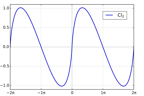
رسم بياني لدالة كلاوسن Cl 2 ( θ ) في الرياضيات ، تُعدّ دالة كلاوسن ، التي قدّمها توماس ( 1832 ) ، دالة خاصة متسامية لمتغير واحد. ويمكن التعبير عنها بصورة تكامل محدد ، أو متسلسلة مثلثية ، أو صيغ أخرى متنوعة. وهي ترتبط ارتباطًا وثيقًا بدالة اللوغاريتم المتعدد ، وتكامل الظل العكسي ، ودالة غاما المتعددة ، ودالة زيتا لريمان ، ودالة إيتا لديريشليه ، ودالة بيتا لديريشليه .
دالة كلاوسن من الرتبة 2 - والتي يشار إليها غالبًا باسم دالة كلاوسن ، على الرغم من كونها واحدة فقط من فئة عديدة - تُعطى بالتكامل التالي:
Cl 2 ( φ ) = - ∫ 0 φ سجل | 2 الخطيئة x 2 | د x {\displaystyle \operatorname {Cl} _{2}(\varphi )=-\int _{0}^{\varphi }\log \left|2\sin {\frac {x}{2}}\right|\,dx}
حيث يرمز log إلى اللوغاريتم الطبيعي . في النطاق0 < φ < 2 π {\displaystyle 0<\varphi <2\pi \,} الجيب داخل علامة القيمة المطلقة موجبة تمامًا، لذا يمكن حذف علامات القيمة المطلقة. كما يمكن تمثيل دالة كلاوسن بمتسلسلة فورييه .
Cl 2 ( φ ) = ∑ ك = 1 ∞ الخطيئة ك φ ك 2 = الخطيئة φ + الخطيئة 2 φ 2 2 + الخطيئة 3 φ 3 2 + الخطيئة 4 φ 4 2 + ⋯ {\displaystyle \operatorname {Cl} _{2}(\varphi)=\sum _{k=1}^{\infty }{\frac {\sin k\varphi }{k^{2}}}=\sin \varphi +{\frac {\sin 2\varphi }{2^{2}}}+{\frac {\sin 3\varphi }{3^{2}}}+{\frac {\sin 4\varphi }{4^{2}}}+\cdots }
تُستخدم دوال كلاوسن، كفئة من الدوال، على نطاق واسع في العديد من مجالات البحث الرياضي الحديث، لا سيما فيما يتعلق بتقييم العديد من فئات التكاملات اللوغاريتمية ومتعددة اللوغاريتمات، سواء المحددة أو غير المحددة. كما أن لها تطبيقات عديدة فيما يتعلق بجمع المتسلسلات فوق الهندسية ، والمجاميع التي تتضمن معكوس معامل ذات الحدين المركزي ، ومجاميع دالة متعددة غاما ، ومتسلسلات ديريشليه L.
الخصائص الأساسية دالة كلاوسن ( من الرتبة 2) لها أصفار بسيطة عند جميع المضاعفات ( الصحيحة ) لـ π ، {\displaystyle \pi ,\,} ك ∈ Z {\displaystyle k\in \mathbb {Z} } الخطيئة ك π = 0 {\displaystyle \sin k\pi =0}
Cl 2 ( م π ) = 0 ، م = 0 ، ± 1 ، ± 2 ، ± 3 ، ⋯ {\displaystyle \operatorname {Cl} _{2}(m\pi )=0,\quad m=0,\,\pm 1,\,\pm 2,\,\pm 3,\,\cdots }
يبلغ ذروته عندθ = π 3 + 2 م π [ م ∈ Z ] {\displaystyle \theta ={\frac {\pi }{3}}+2m\pi \quad [m\in \mathbb {Z} ]}
Cl 2 ( π 3 + 2 م π ) = 1.01494160 ... {\displaystyle \operatorname {Cl} _{2}\left({\frac {\pi }{3}}+2m\pi \right)=1.01494160\ldots }
والحد الأدنى عندθ = - π 3 + 2 م π [ م ∈ Z ] {\displaystyle \theta =-{\frac {\pi }{3}}+2m\pi \quad [m\in \mathbb {Z} ]}
Cl 2 ( - π 3 + 2 م π ) = - 1.01494160 ... {\displaystyle \operatorname {Cl} _{2}\left(-{\frac {\pi }{3}}+2m\pi \right)=-1.01494160\ldots }
الخصائص التالية هي نتائج مباشرة لتعريف السلسلة:
Cl 2 ( θ + 2 م π ) = Cl 2 ( θ ) {\displaystyle \operatorname {Cl} _{2}(\theta +2m\pi )=\operatorname {Cl} _{2}(\theta )} Cl 2 ( - θ ) = - Cl 2 ( θ ) {\displaystyle \operatorname {Cl} _{2}(-\theta )=-\operatorname {Cl} _{2}(\theta )}
انظر لو وبيريز (1992) .
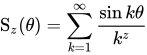
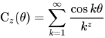
التعريف العام وبشكل أعم، يتم تعريف دالتي كلاوسن المعممتين:
S z ( θ ) = ∑ ك = 1 ∞ الخطيئة ك θ ك z {\displaystyle \operatorname {S} _{z}(\theta )=\sum _{k=1}^{\infty }{\frac {\sin k\theta} {k^{z}}}} ج z ( θ ) = ∑ ك = 1 ∞ كوس ك θ ك z {\displaystyle \operatorname {C} _{z}(\theta )=\sum _{k=1}^{\infty }{\frac {\cos k\theta} {k^{z}}}}
والتي تكون صالحة للأعداد المركبة z مع Re z > 1. ويمكن توسيع التعريف ليشمل جميع المستويات المركبة من خلال الاستمرار التحليلي .
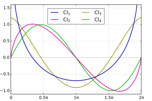
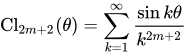
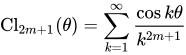
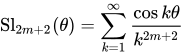
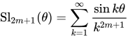
When z is replaced with a non-negative integer, the standard Clausen functions are defined by the following Fourier series :
Cl 2 m + 2 ( θ ) = ∑ k = 1 ∞ sin k θ k 2 m + 2 {\displaystyle \operatorname {Cl} _{2m+2}(\theta )=\sum _{k=1}^{\infty }{\frac {\sin k\theta }{k^{2m+2}}}} Cl 2 m + 1 ( θ ) = ∑ k = 1 ∞ cos k θ k 2 m + 1 {\displaystyle \operatorname {Cl} _{2m+1}(\theta )=\sum _{k=1}^{\infty }{\frac {\cos k\theta }{k^{2m+1}}}} Sl 2 m + 2 ( θ ) = ∑ k = 1 ∞ cos k θ k 2 m + 2 {\displaystyle \operatorname {Sl} _{2m+2}(\theta )=\sum _{k=1}^{\infty }{\frac {\cos k\theta }{k^{2m+2}}}} Sl 2 m + 1 ( θ ) = ∑ k = 1 ∞ sin k θ k 2 m + 1 {\displaystyle \operatorname {Sl} _{2m+1}(\theta )=\sum _{k=1}^{\infty }{\frac {\sin k\theta }{k^{2m+1}}}}
N.B. The SL-type Clausen functions have the alternative notation Gl m ( θ ) {\displaystyle \operatorname {Gl} _{m}(\theta )\,} Glaisher–Clausen functions (after James Whitbread Lee Glaisher , hence the GL-notation).
Relation to the Bernoulli polynomials The SL-type Clausen function are polynomials in θ {\displaystyle \,\theta \,} Bernoulli polynomials . This connection is apparent from the Fourier series representations of the Bernoulli polynomials:
B 2 n − 1 ( x ) = 2 ( − 1 ) n ( 2 n − 1 ) ! ( 2 π ) 2 n − 1 ∑ k = 1 ∞ sin 2 π k x k 2 n − 1 . {\displaystyle B_{2n-1}(x)={\frac {2(-1)^{n}(2n-1)!}{(2\pi )^{2n-1}}}\,\sum _{k=1}^{\infty }{\frac {\sin 2\pi kx}{k^{2n-1}}}.} B 2 n ( x ) = 2 ( − 1 ) n − 1 ( 2 n ) ! ( 2 π ) 2 n ∑ k = 1 ∞ cos 2 π k x k 2 n . {\displaystyle B_{2n}(x)={\frac {2(-1)^{n-1}(2n)!}{(2\pi )^{2n}}}\,\sum _{k=1}^{\infty }{\frac {\cos 2\pi kx}{k^{2n}}}.}
Setting x = θ / 2 π {\displaystyle \,x=\theta /2\pi \,}
Sl 2 m ( θ ) = ( − 1 ) m − 1 ( 2 π ) 2 m 2 ( 2 m ) ! B 2 m ( θ 2 π ) , {\displaystyle \operatorname {Sl} _{2m}(\theta )={\frac {(-1)^{m-1}(2\pi )^{2m}}{2(2m)!}}B_{2m}\left({\frac {\theta }{2\pi }}\right),} Sl 2 m − 1 ( θ ) = ( − 1 ) m ( 2 π ) 2 m − 1 2 ( 2 m − 1 ) ! B 2 m − 1 ( θ 2 π ) , {\displaystyle \operatorname {Sl} _{2m-1}(\theta )={\frac {(-1)^{m}(2\pi )^{2m-1}}{2(2m-1)!}}B_{2m-1}\left({\frac {\theta }{2\pi }}\right),}
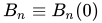
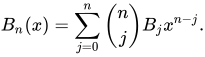
where the Bernoulli polynomials B n ( x ) {\displaystyle \,B_{n}(x)\,} Bernoulli numbers B n ≡ B n ( 0 ) {\displaystyle \,B_{n}\equiv B_{n}(0)\,}
B n ( x ) = ∑ j = 0 n ( n j ) B j x n − j . {\displaystyle B_{n}(x)=\sum _{j=0}^{n}{\binom {n}{j}}B_{j}x^{n-j}.}
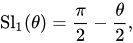
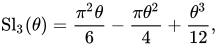
Explicit evaluations derived from the above include:
Sl 1 ( θ ) = π 2 − θ 2 , {\displaystyle \operatorname {Sl} _{1}(\theta )={\frac {\pi }{2}}-{\frac {\theta }{2}},} Sl 2 ( θ ) = π 2 6 − π θ 2 + θ 2 4 , {\displaystyle \operatorname {Sl} _{2}(\theta )={\frac {\pi ^{2}}{6}}-{\frac {\pi \theta }{2}}+{\frac {\theta ^{2}}{4}},} Sl 3 ( θ ) = π 2 θ 6 − π θ 2 4 + θ 3 12 , {\displaystyle \operatorname {Sl} _{3}(\theta )={\frac {\pi ^{2}\theta }{6}}-{\frac {\pi \theta ^{2}}{4}}+{\frac {\theta ^{3}}{12}},} Sl 4 ( θ ) = π 4 90 − π 2 θ 2 12 + π θ 3 12 − θ 4 48 . {\displaystyle \operatorname {Sl} _{4}(\theta )={\frac {\pi ^{4}}{90}}-{\frac {\pi ^{2}\theta ^{2}}{12}}+{\frac {\pi \theta ^{3}}{12}}-{\frac {\theta ^{4}}{48}}.}
For 0 < θ < π {\displaystyle 0<\theta <\pi } Lu & Perez (1992) for the result – although no proof is given):
Cl 2 ( 2 θ ) = 2 Cl 2 ( θ ) − 2 Cl 2 ( π − θ ) {\displaystyle \operatorname {Cl} _{2}(2\theta )=2\operatorname {Cl} _{2}(\theta )-2\operatorname {Cl} _{2}(\pi -\theta )}
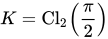
Denoting Catalan's constant by K = Cl 2 ( π 2 ) {\displaystyle K=\operatorname {Cl} _{2}\left({\frac {\pi }{2}}\right)}
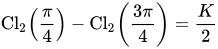
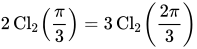
Cl 2 ( π 4 ) − Cl 2 ( 3 π 4 ) = K 2 {\displaystyle \operatorname {Cl} _{2}\left({\frac {\pi }{4}}\right)-\operatorname {Cl} _{2}\left({\frac {3\pi }{4}}\right)={\frac {K}{2}}} 2 Cl 2 ( π 3 ) = 3 Cl 2 ( 2 π 3 ) {\displaystyle 2\operatorname {Cl} _{2}\left({\frac {\pi }{3}}\right)=3\operatorname {Cl} _{2}\left({\frac {2\pi }{3}}\right)}
For higher order Clausen functions, duplication formulae can be obtained from the one given above; simply replace θ {\displaystyle \,\theta \,} dummy variable x {\displaystyle x} [ 0 , θ ] . {\displaystyle \,[0,\theta ].\,}
Cl 3 ( 2 θ ) = 4 Cl 3 ( θ ) + 4 Cl 3 ( π − θ ) {\displaystyle \operatorname {Cl} _{3}(2\theta )=4\operatorname {Cl} _{3}(\theta )+4\operatorname {Cl} _{3}(\pi -\theta )} Cl 4 ( 2 θ ) = 8 Cl 4 ( θ ) − 8 Cl 4 ( π − θ ) {\displaystyle \operatorname {Cl} _{4}(2\theta )=8\operatorname {Cl} _{4}(\theta )-8\operatorname {Cl} _{4}(\pi -\theta )} Cl 5 ( 2 θ ) = 16 Cl 5 ( θ ) + 16 Cl 5 ( π − θ ) {\displaystyle \operatorname {Cl} _{5}(2\theta )=16\operatorname {Cl} _{5}(\theta )+16\operatorname {Cl} _{5}(\pi -\theta )} Cl 6 ( 2 θ ) = 32 Cl 6 ( θ ) − 32 Cl 6 ( π − θ ) {\displaystyle \operatorname {Cl} _{6}(2\theta )=32\operatorname {Cl} _{6}(\theta )-32\operatorname {Cl} _{6}(\pi -\theta )}
And more generally, upon induction on m , m ≥ 1 {\displaystyle \,m,\;m\geq 1}
Cl m + 1 ( 2 θ ) = 2 m [ Cl m + 1 ( θ ) + ( − 1 ) m Cl m + 1 ( π − θ ) ] {\displaystyle \operatorname {Cl} _{m+1}(2\theta )=2^{m}\left[\operatorname {Cl} _{m+1}(\theta )+(-1)^{m}\operatorname {Cl} _{m+1}(\pi -\theta )\right]}
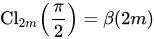
Use of the generalized duplication formula allows for an extension of the result for the Clausen function of order 2, involving Catalan's constant . For m ∈ Z ≥ 1 {\displaystyle \,m\in \mathbb {Z} \geq 1\,}
Cl 2 m ( π 2 ) = 2 2 m − 1 [ Cl 2 m ( π 4 ) − Cl 2 m ( 3 π 4 ) ] = β ( 2 m ) {\displaystyle \operatorname {Cl} _{2m}\left({\frac {\pi }{2}}\right)=2^{2m-1}\left[\operatorname {Cl} _{2m}\left({\frac {\pi }{4}}\right)-\operatorname {Cl} _{2m}\left({\frac {3\pi }{4}}\right)\right]=\beta (2m)}
Where β ( x ) {\displaystyle \,\beta (x)\,} Dirichlet beta function .
From the integral definition,
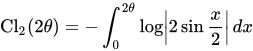
Cl 2 ( 2 θ ) = − ∫ 0 2 θ log | 2 sin x 2 | d x {\displaystyle \operatorname {Cl} _{2}(2\theta )=-\int _{0}^{2\theta }\log \left|2\sin {\frac {x}{2}}\right|\,dx}
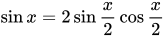
Apply the duplication formula for the sine function , sin x = 2 sin x 2 cos x 2 {\displaystyle \sin x=2\sin {\frac {x}{2}}\cos {\frac {x}{2}}}
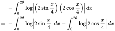
− ∫ 0 2 θ log | ( 2 sin x 4 ) ( 2 cos x 4 ) | d x = − ∫ 0 2 θ log | 2 sin x 4 | d x − ∫ 0 2 θ log | 2 cos x 4 | d x {\displaystyle {\begin{aligned}&-\int _{0}^{2\theta }\log \left|\left(2\sin {\frac {x}{4}}\right)\left(2\cos {\frac {x}{4}}\right)\right|\,dx\\={}&-\int _{0}^{2\theta }\log \left|2\sin {\frac {x}{4}}\right|\,dx-\int _{0}^{2\theta }\log \left|2\cos {\frac {x}{4}}\right|\,dx\end{aligned}}}
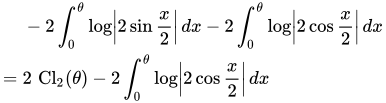
Apply the substitution x = 2 y , d x = 2 d y {\displaystyle x=2y,dx=2\,dy}
− 2 ∫ 0 θ log | 2 sin x 2 | d x − 2 ∫ 0 θ log | 2 cos x 2 | d x = 2 Cl 2 ( θ ) − 2 ∫ 0 θ log | 2 cos x 2 | d x {\displaystyle {\begin{aligned}&-2\int _{0}^{\theta }\log \left|2\sin {\frac {x}{2}}\right|\,dx-2\int _{0}^{\theta }\log \left|2\cos {\frac {x}{2}}\right|\,dx\\={}&2\,\operatorname {Cl} _{2}(\theta )-2\int _{0}^{\theta }\log \left|2\cos {\frac {x}{2}}\right|\,dx\end{aligned}}}
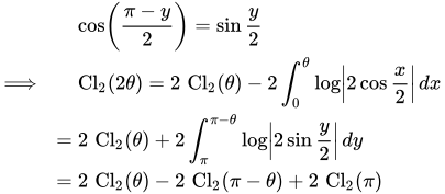
On that last integral, set y = π − x , x = π − y , d x = − d y {\displaystyle y=\pi -x,\,x=\pi -y,\,dx=-dy} cos ( x − y ) = cos x cos y − sin x sin y {\displaystyle \cos(x-y)=\cos x\cos y-\sin x\sin y}
cos ( π − y 2 ) = sin y 2 ⟹ Cl 2 ( 2 θ ) = 2 Cl 2 ( θ ) − 2 ∫ 0 θ log | 2 cos x 2 | d x = 2 Cl 2 ( θ ) + 2 ∫ π π − θ log | 2 sin y 2 | d y = 2 Cl 2 ( θ ) − 2 Cl 2 ( π − θ ) + 2 Cl 2 ( π ) {\displaystyle {\begin{aligned}&\cos \left({\frac {\pi -y}{2}}\right)=\sin {\frac {y}{2}}\\\Longrightarrow \qquad &\operatorname {Cl} _{2}(2\theta )=2\,\operatorname {Cl} _{2}(\theta )-2\int _{0}^{\theta }\log \left|2\cos {\frac {x}{2}}\right|\,dx\\={}&2\,\operatorname {Cl} _{2}(\theta )+2\int _{\pi }^{\pi -\theta }\log \left|2\sin {\frac {y}{2}}\right|\,dy\\={}&2\,\operatorname {Cl} _{2}(\theta )-2\,\operatorname {Cl} _{2}(\pi -\theta )+2\,\operatorname {Cl} _{2}(\pi )\end{aligned}}} Cl 2 ( π ) = 0 {\displaystyle \operatorname {Cl} _{2}(\pi )=0\,} Therefore,
Cl 2 ( 2 θ ) = 2 Cl 2 ( θ ) − 2 Cl 2 ( π − θ ) . ◻ {\displaystyle \operatorname {Cl} _{2}(2\theta )=2\,\operatorname {Cl} _{2}(\theta )-2\,\operatorname {Cl} _{2}(\pi -\theta )\,.\,\Box }
Derivatives of general-order Clausen functions Direct differentiation of the Fourier series expansions for the Clausen functions give:
d d θ Cl 2 m + 2 ( θ ) = d d θ ∑ k = 1 ∞ sin k θ k 2 m + 2 = ∑ k = 1 ∞ cos k θ k 2 m + 1 = Cl 2 m + 1 ( θ ) {\displaystyle {\frac {d}{d\theta }}\operatorname {Cl} _{2m+2}(\theta )={\frac {d}{d\theta }}\sum _{k=1}^{\infty }{\frac {\sin k\theta }{k^{2m+2}}}=\sum _{k=1}^{\infty }{\frac {\cos k\theta }{k^{2m+1}}}=\operatorname {Cl} _{2m+1}(\theta )} d d θ Cl 2 m + 1 ( θ ) = d d θ ∑ k = 1 ∞ cos k θ k 2 m + 1 = − ∑ k = 1 ∞ sin k θ k 2 m = − Cl 2 m ( θ ) {\displaystyle {\frac {d}{d\theta }}\operatorname {Cl} _{2m+1}(\theta )={\frac {d}{d\theta }}\sum _{k=1}^{\infty }{\frac {\cos k\theta }{k^{2m+1}}}=-\sum _{k=1}^{\infty }{\frac {\sin k\theta }{k^{2m}}}=-\operatorname {Cl} _{2m}(\theta )} d d θ Sl 2 m + 2 ( θ ) = d d θ ∑ k = 1 ∞ cos k θ k 2 m + 2 = − ∑ k = 1 ∞ sin k θ k 2 m + 1 = − Sl 2 m + 1 ( θ ) {\displaystyle {\frac {d}{d\theta }}\operatorname {Sl} _{2m+2}(\theta )={\frac {d}{d\theta }}\sum _{k=1}^{\infty }{\frac {\cos k\theta }{k^{2m+2}}}=-\sum _{k=1}^{\infty }{\frac {\sin k\theta }{k^{2m+1}}}=-\operatorname {Sl} _{2m+1}(\theta )} d d θ Sl 2 m + 1 ( θ ) = d d θ ∑ k = 1 ∞ sin k θ k 2 m + 1 = ∑ k = 1 ∞ cos k θ k 2 m = Sl 2 m ( θ ) {\displaystyle {\frac {d}{d\theta }}\operatorname {Sl} _{2m+1}(\theta )={\frac {d}{d\theta }}\sum _{k=1}^{\infty }{\frac {\sin k\theta }{k^{2m+1}}}=\sum _{k=1}^{\infty }{\frac {\cos k\theta }{k^{2m}}}=\operatorname {Sl} _{2m}(\theta )}
By appealing to the First Fundamental Theorem Of Calculus , we also have:
d d θ Cl 2 ( θ ) = d d θ [ − ∫ 0 θ log | 2 sin x 2 | d x ] = − log | 2 sin θ 2 | = Cl 1 ( θ ) {\displaystyle {\frac {d}{d\theta }}\operatorname {Cl} _{2}(\theta )={\frac {d}{d\theta }}\left[-\int _{0}^{\theta }\log \left|2\sin {\frac {x}{2}}\right|\,dx\,\right]=-\log \left|2\sin {\frac {\theta }{2}}\right|=\operatorname {Cl} _{1}(\theta )}
Relation to the inverse tangent integral The inverse tangent integral is defined on the interval 0 < z < 1 {\displaystyle 0<z<1}
Ti 2 ( z ) = ∫ 0 z tan − 1 x x d x = ∑ k = 0 ∞ ( − 1 ) k z 2 k + 1 ( 2 k + 1 ) 2 {\displaystyle \operatorname {Ti} _{2}(z)=\int _{0}^{z}{\frac {\tan ^{-1}x}{x}}\,dx=\sum _{k=0}^{\infty }(-1)^{k}{\frac {z^{2k+1}}{(2k+1)^{2}}}}
It has the following closed form in terms of the Clausen function:
Ti 2 ( tan θ ) = θ log ( tan θ ) + 1 2 Cl 2 ( 2 θ ) + 1 2 Cl 2 ( π − 2 θ ) {\displaystyle \operatorname {Ti} _{2}(\tan \theta )=\theta \log(\tan \theta )+{\frac {1}{2}}\operatorname {Cl} _{2}(2\theta )+{\frac {1}{2}}\operatorname {Cl} _{2}(\pi -2\theta )}
Proof of the inverse tangent integral relation من التعريف التكاملي للتكامل العكسي للظل ، لدينا
تي 2 ( لون برونزي θ ) = ∫ 0 لون برونزي θ لون برونزي - 1 x x د x {\displaystyle \operatorname {Ti} _{2}(\tan \theta )=\int _{0}^{\tan \theta }{\frac {\tan ^{-1}x}{x}}\,dx}
إجراء التكامل بالتجزئة
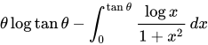
∫ 0 لون برونزي θ لون برونزي - 1 x x د x = لون برونزي - 1 x سجل x | 0 لون برونزي θ - ∫ 0 لون برونزي θ سجل x 1 + x 2 د x = {\displaystyle \int _{0}^{\tan \theta }{\frac {\tan ^{-1}x}{x}}\,dx=\tan ^{-1}x\log x\,{\Bigg |}_{0}^{\tan \theta }-\int _{0}^{\tan \theta }{\frac {\log x}{1+x^{2}}}\,dx=} θ سجل لون برونزي θ - ∫ 0 لون برونزي θ سجل x 1 + x 2 د x {\displaystyle \theta \log \tan \theta -\int _{0}^{\tan \theta }{\frac {\log x}{1+x^{2}}}\,dx}
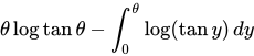
قم بتطبيق الاستبدالx = لون برونزي y ، y = لون برونزي - 1 x ، د y = د x 1 + x 2 {\displaystyle x=\tan y,\,y=\tan ^{-1}x,\,dy={\frac {dx}{1+x^{2}}}\,}
θ سجل لون برونزي θ - ∫ 0 θ سجل ( لون برونزي y ) د y {\displaystyle \theta \log \tan \theta -\int _{0}^{\theta }\log(\tan y)\,dy}
بالنسبة للتكامل الأخير، قم بتطبيق التحويلy = x / 2 ، د y = د x / 2 {\displaystyle y=x/2,\,dy=dx/2\,}
θ سجل لون برونزي θ - 1 2 ∫ 0 2 θ سجل ( لون برونزي x 2 ) د x = θ سجل لون برونزي θ - 1 2 ∫ 0 2 θ سجل ( الخطيئة ( x / 2 ) كوس ( x / 2 ) ) د x = θ سجل لون برونزي θ - 1 2 ∫ 0 2 θ سجل ( 2 الخطيئة ( x / 2 ) 2 كوس ( x / 2 ) ) د x = θ سجل لون برونزي θ - 1 2 ∫ 0 2 θ سجل ( 2 الخطيئة x 2 ) د x + 1 2 ∫ 0 2 θ سجل ( 2 كوس x 2 ) د x = θ سجل لون برونزي θ + 1 2 Cl 2 ( 2 θ ) + 1 2 ∫ 0 2 θ سجل ( 2 كوس x 2 ) د x . {\displaystyle {\begin{aligned}&\theta \log \tan \theta -{\frac {1}{2}}\int _{0}^{2\theta }\log \left(\tan {\frac {x}{2}}\right)\,dx\\[6pt]={}&\theta \log \tan \theta -{\frac {1}{2}}\int _{0}^{2\theta }\log \left({\frac {\sin(x/2)}{\cos(x/2)}}\right)\,dx\\[6pt]={}&\theta \log \tan \theta -{\frac {1}{2}}\int _{0}^{2\theta }\log \left({\frac {2\sin(x/2)}{2\cos(x/2)}}\right)\,dx\\[6pt]={}&\theta \log \tan \theta -{\frac {1}{2}}\int _{0}^{2\theta }\log \left(2\sin {\frac {x}{2}}\right)\,dx+{\frac {1}{2}}\int _{0}^{2\theta }\log \left(2\cos {\frac {x}{2}}\right)\,dx\\[6pt]={}&\theta \log \tan \theta +{\frac {1}{2}}\operatorname {Cl} _{2}(2\theta )+{\frac {1}{2}}\int _{0}^{2\theta }\log \left(2\cos {\frac {x}{2}}\right)\,dx.\end{aligned}}}
وأخيرًا، كما هو الحال مع برهان صيغة التكرار، فإن الاستبدالx = ( π - y ) {\displaystyle x=(\pi -y)\,}
∫ 0 2 θ سجل ( 2 كوس x 2 ) د x = Cl 2 ( π - 2 θ ) - Cl 2 ( π ) = Cl 2 ( π - 2 θ ) {\displaystyle \int _{0}^{2\theta }\log \left(2\cos {\frac {x}{2}}\right)\,dx=\operatorname {Cl} _{2}(\pi -2\theta )-\operatorname {Cl} _{2}(\pi )=\operatorname {Cl} _{2}(\pi -2\theta )}
هكذا
تي 2 ( لون برونزي θ ) = θ سجل لون برونزي θ + 1 2 Cl 2 ( 2 θ ) + 1 2 Cl 2 ( π - 2 θ ) . ◻ {\displaystyle \operatorname {Ti} _{2}(\tan \theta )=\theta \log \tan \theta +{\frac {1}{2}}\operatorname {Cl} _{2}(2\theta )+{\frac {1}{2}}\operatorname {Cl} _{2}(\pi -2\theta )\,.\,\Box }
لريال مدريد0 < z < 1 {\displaystyle 0<z<1} دالة بارنز G ودالة غاما (أويلر) :
Cl 2 ( 2 π z ) = 2 π سجل ( جي ( 1 - z ) جي ( 1 + z ) ) + 2 π z سجل ( π الخطيئة π z ) {\displaystyle \operatorname {Cl} _{2}(2\pi z)=2\pi \log \left({\frac {G(1-z)}{G(1+z)}}\right)+2\pi z\log \left({\frac {\pi }{\sin \pi z}}\right)}
أو ما يعادل ذلك
Cl 2 ( 2 π z ) = 2 π سجل ( جي ( 1 - z ) جي ( z ) ) - 2 π سجل Γ ( z ) + 2 π z سجل ( π الخطيئة π z ) {\displaystyle \operatorname {Cl} _{2}(2\pi z)=2\pi \log \left({\frac {G(1-z)}{G(z)}}\right)-2\pi \log \Gamma (z)+2\pi z\log \left({\frac {\pi }{\sin \pi z}}\right)}
انظر آدمشيك (2003) .
العلاقة باللوغاريتم المتعدد تمثل دوال كلاوسن الأجزاء الحقيقية والخيالية للوغاريتم المتعدد، على دائرة الوحدة :
Cl 2 م ( θ ) = ℑ ( لي 2 م ( هـ أنا θ ) ) ، م ∈ Z ≥ 1 {\displaystyle \operatorname {Cl} _{2m}(\theta )=\Im (\operatorname {Li} _{2m}(e^{i\theta })),\quad m\in \mathbb {Z} \geq 1} Cl 2 م + 1 ( θ ) = ℜ ( لي 2 م + 1 ( هـ أنا θ ) ) ، م ∈ Z ≥ 0 {\displaystyle \operatorname {Cl} _{2m+1}(\theta )=\Re (\operatorname {Li} _{2m+1}(e^{i\theta })),\quad m\in \mathbb {Z} \geq 0}
ويمكن ملاحظة ذلك بسهولة من خلال الرجوع إلى تعريف المتسلسلة للوغاريتم المتعدد .
لي ن ( z ) = ∑ ك = 1 ∞ z ك ك ن ⟹ لي ن ( هـ أنا θ ) = ∑ ك = 1 ∞ ( هـ أنا θ ) ك ك ن = ∑ ك = 1 ∞ هـ أنا ك θ ك ن {\displaystyle \operatorname {Li} _{n}(z)=\sum _{k=1}^{\infty }{\frac {z^{k}}{k^{n}}}\quad \Longrightarrow \operatorname {Li} _{n}\left(e^{i\theta }\right)=\sum _{k=1}^{\infty }{\frac {\left(e^{i\theta }\right)^{k}}{k^{n}}}=\sum _{k=1}^{\infty }{\frac {e^{ik\theta }}{k^{n}}}}
بحسب نظرية أويلر،
هـ أنا θ = كوس θ + أنا الخطيئة θ {\displaystyle e^{i\theta }=\cos \theta +i\sin \theta }
وبواسطة نظرية دي موافر ( صيغة دي موافر )
( كوس θ + أنا الخطيئة θ ) ك = كوس ك θ + أنا الخطيئة ك θ ⇒ لي ن ( هـ أنا θ ) = ∑ ك = 1 ∞ كوس ك θ ك ن + أنا ∑ ك = 1 ∞ الخطيئة ك θ ك ن {\displaystyle (\cos \theta +i\sin \theta )^{k}=\cos k\theta +i\sin k\theta \quad \Rightarrow \operatorname {Li} _{n}\left(e^{i\theta }\right)=\sum _{k=1}^{\infty }{\frac {\cos k\theta }{k^{n}}}+i\,\sum _{k=1}^{\infty }{\frac {\sin k\theta }{k^{n}}}}
لذلك
لي 2 م ( هـ أنا θ ) = ∑ ك = 1 ∞ كوس ك θ ك 2 م + أنا ∑ ك = 1 ∞ الخطيئة ك θ ك 2 م = سل 2 م ( θ ) + أنا Cl 2 م ( θ ) {\displaystyle \operatorname {Li} _{2m}\left(e^{i\theta }\right)=\sum _{k=1}^{\infty }{\frac {\cos k\theta }{k^{2m}}}+i\,\sum _{k=1}^{\infty }{\frac {\sin k\theta }{k^{2m}}}=\operatorname {Sl} _{2m}(\theta )+i\operatorname {Cl} _{2m}(\theta )} لي 2 م + 1 ( هـ أنا θ ) = ∑ ك = 1 ∞ كوس ك θ ك 2 م + 1 + أنا ∑ ك = 1 ∞ الخطيئة ك θ ك 2 م + 1 = Cl 2 م + 1 ( θ ) + أنا سل 2 م + 1 ( θ ) {\displaystyle \operatorname {Li} _{2m+1}\left(e^{i\theta }\right)=\sum _{k=1}^{\infty }{\frac {\cos k\theta }{k^{2m+1}}}+i\,\sum _{k=1}^{\infty }{\frac {\sin k\theta }{k^{2m+1}}}=\operatorname {Cl} _{2m+1}(\theta )+i\operatorname {Sl} _{2m+1}(\theta )}
العلاقة بدالة بوليغاما ترتبط دوال كلاوسن ارتباطًا وثيقًا بدالة بوليغاما . في الواقع، من الممكن التعبير عن دوال كلاوسن كتركيبات خطية من دوال الجيب ودوال بوليغاما. إحدى هذه العلاقات موضحة هنا، ومثبتة أدناه:
Cl 2 م ( q π ص ) = 1 ( 2 ص ) 2 م ( 2 م - 1 ) ! ∑ ج = 1 ص الخطيئة ( q ج π ص ) [ ψ 2 م - 1 ( ج 2 ص ) + ( - 1 ) q ψ 2 م - 1 ( ج + ص 2 ص ) ] . {\displaystyle \operatorname {Cl} _{2m}\left({\frac {q\pi }{p}}\right)={\frac {1}{(2p)^{2m}(2m-1)!}}\,\sum _{j=1}^{p}\sin \left({\tfrac {qj\pi }{p}}\right)\,\left[\psi _{2m-1}\left({\tfrac {j}{2p}}\right)+(-1)^{q}\psi _{2m-1}\left({\tfrac {j+p}{2p}}\right)\right].}
والنتيجة المباشرة لذلك هي هذه الصيغة المكافئة بدلالة دالة زيتا لهورويتز:
Cl 2 م ( q π ص ) = 1 ( 2 ص ) 2 م ∑ ج = 1 ص الخطيئة ( q ج π ص ) [ ζ ( 2 م ، ج 2 ص ) + ( - 1 ) q ζ ( 2 م ، ج + ص 2 ص ) ] . {\displaystyle \operatorname {Cl} _{2m}\left({\frac {q\pi }{p}}\right)={\frac {1}{(2p)^{2m}}}\,\sum _{j=1}^{p}\sin \left({\tfrac {qj\pi }{p}}\right)\,\left[\zeta \left(2m,{\tfrac {j}{2p}}\right)+(-1)^{q}\zeta \left(2m,{\tfrac {j+p}{2p}}\right)\right].}
إثبات الصيغة
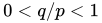
يتركص {\displaystyle \,p\,} q {\displaystyle \,q\,} q / ص {\displaystyle \,q/p\,} 0 < q / ص < 1 {\displaystyle \,0<q/p<1\,}
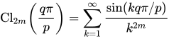
Cl 2 م ( q π ص ) = ∑ ك = 1 ∞ الخطيئة ( ك q π / ص ) ك 2 م {\displaystyle \operatorname {Cl} _{2m}\left({\frac {q\pi }{p}}\right)=\sum _{k=1}^{\infty }{\frac {\sin(kq\pi /p)}{k^{2m}}}}
نقسم هذا المجموع إلى p جزءًا بالضبط، بحيث تحتوي السلسلة الأولى على جميع الحدود المتطابقة مع، وفقط، تلك الحدود المتطابقة معك ص + 1 ، {\displaystyle \,kp+1,\,} ك ص + 2 ، {\displaystyle \,kp+2,\,} p ، الذي يحتوي على جميع الحدود المتطابقة معك ص + ص {\displaystyle \,kp+p\,}
Cl 2 م ( q π ص ) = ∑ ك = 0 ∞ الخطيئة [ ( ك ص + 1 ) q π ص ] ( ك ص + 1 ) 2 م + ∑ ك = 0 ∞ الخطيئة [ ( ك ص + 2 ) q π ص ] ( ك ص + 2 ) 2 م + ∑ ك = 0 ∞ الخطيئة [ ( ك ص + 3 ) q π ص ] ( ك ص + 3 ) 2 م + ⋯ ⋯ + ∑ ك = 0 ∞ الخطيئة [ ( ك ص + ص - 2 ) q π ص ] ( ك ص + ص - 2 ) 2 م + ∑ ك = 0 ∞ الخطيئة [ ( ك ص + ص - 1 ) q π ص ] ( ك ص + ص - 1 ) 2 م + ∑ ك = 0 ∞ الخطيئة [ ( ك ص + ص ) q π ص ] ( ك ص + ص ) 2 م {\displaystyle {\begin{aligned}&\operatorname {Cl} _{2m}\left({\frac {q\pi }{p}}\right)\\={}&\sum _{k=0}^{\infty }{\frac {\sin \left[(kp+1){\frac {q\pi }{p}}\right]}{(kp+1)^{2m}}}+\sum _{k=0}^{\infty }{\frac {\sin \left[(kp+2){\frac {q\pi }{p}}\right]}{(kp+2)^{2m}}}+\sum _{k=0}^{\infty }{\frac {\sin \left[(kp+3){\frac {q\pi }{p}}\right]}{(kp+3)^{2m}}}+\cdots \\&\cdots +\sum _{k=0}^{\infty }{\frac {\sin \left[(kp+p-2){\frac {q\pi }{p}}\right]}{(kp+p-2)^{2m}}}+\sum _{k=0}^{\infty }{\frac {\sin \left[(kp+p-1){\frac {q\pi }{p}}\right]}{(kp+p-1)^{2m}}}+\sum _{k=0}^{\infty }{\frac {\sin \left[(kp+p){\frac {q\pi }{p}}\right]}{(kp+p)^{2m}}}\end{aligned}}}
يمكننا فهرسة هذه المجاميع لتشكيل مجموع مزدوج:
Cl 2 م ( q π ص ) = ∑ ج = 1 ص { ∑ ك = 0 ∞ الخطيئة [ ( ك ص + ج ) q π ص ] ( ك ص + ج ) 2 م } = ∑ ج = 1 ص 1 ص 2 م { ∑ ك = 0 ∞ الخطيئة [ ( ك ص + ج ) q π ص ] ( ك + ( ج / ص ) ) 2 م } {\displaystyle {\begin{aligned}&\operatorname {Cl} _{2m}\left({\frac {q\pi }{p}}\right)=\sum _{j=1}^{p}\left\{\sum _{k=0}^{\infty }{\frac {\sin \left[(kp+j){\frac {q\pi }{p}}\right]}{(kp+j)^{2m}}}\right\}\\={}&\sum _{j=1}^{p}{\frac {1}{p^{2m}}}\left\{\sum _{k=0}^{\infty }{\frac {\sin \left[(kp+j){\frac {q\pi }{p}}\right]}{(k+(j/p))^{2m}}}\right\}\end{aligned}}}
بتطبيق صيغة الجمع لدالة الجيب ،الخطيئة ( x + y ) = الخطيئة x كوس y + كوس x الخطيئة y ، {\displaystyle \,\sin(x+y)=\sin x\cos y+\cos x\sin y,\,}
الخطيئة [ ( ك ص + ج ) q π ص ] = الخطيئة ( ك q π + q ج π ص ) = الخطيئة ك q π كوس q ج π ص + كوس ك q π الخطيئة q ج π ص {\displaystyle \sin \left[(kp+j){\frac {q\pi }{p}}\right]=\sin \left(kq\pi +{\frac {qj\pi }{p}}\right)=\sin kq\pi \cos {\frac {qj\pi }{p}}+\cos kq\pi \sin {\frac {qj\pi }{p}}} الخطيئة م π ≡ 0 ، كوس م π ≡ ( - 1 ) م ⟺ م = 0 ، ± 1 ، ± 2 ، ± 3 ، ... {\displaystyle \sin m\pi \equiv 0,\quad \,\cos m\pi \equiv (-1)^{m}\quad \Longleftrightarrow m=0,\,\pm 1,\,\pm 2,\,\pm 3,\,\ldots } الخطيئة [ ( ك ص + ج ) q π ص ] = ( - 1 ) ك q الخطيئة q ج π ص {\displaystyle \sin \left[(kp+j){\frac {q\pi }{p}}\right]=(-1)^{kq}\sin {\frac {qj\pi }{p}}}
بالتالي،
Cl 2 م ( q π ص ) = ∑ ج = 1 ص 1 ص 2 م الخطيئة ( q ج π ص ) { ∑ ك = 0 ∞ ( - 1 ) ك q ( ك + ( ج / ص ) ) 2 م } {\displaystyle \operatorname {Cl} _{2m}\left({\frac {q\pi }{p}}\right)=\sum _{j=1}^{p}{\frac {1}{p^{2m}}}\sin \left({\frac {qj\pi }{p}}\right)\,\left\{\sum _{k=0}^{\infty }{\frac {(-1)^{kq}}{(k+(j/p))^{2m}}}\right\}}
لتحويل المجموع الداخلي في المجموع المزدوج إلى مجموع غير متناوب، قم بتقسيمه إلى جزأين بنفس الطريقة التي تم بها تقسيم المجموع السابق إلى أجزاء p :
∑ ك = 0 ∞ ( - 1 ) ك q ( ك + ( ج / ص ) ) 2 م = ∑ ك = 0 ∞ ( - 1 ) ( 2 ك ) q ( ( 2 ك ) + ( ج / ص ) ) 2 م + ∑ ك = 0 ∞ ( - 1 ) ( 2 ك + 1 ) q ( ( 2 ك + 1 ) + ( ج / ص ) ) 2 م = ∑ ك = 0 ∞ 1 ( 2 ك + ( ج / ص ) ) 2 م + ( - 1 ) q ∑ ك = 0 ∞ 1 ( 2 ك + 1 + ( ج / ص ) ) 2 م = 1 2 ص [ ∑ ك = 0 ∞ 1 ( ك + ( ج / 2 ص ) ) 2 م + ( - 1 ) q ∑ ك = 0 ∞ 1 ( ك + ( ج + ص 2 ص ) ) 2 م ] {\displaystyle {\begin{aligned}&\sum _{k=0}^{\infty }{\frac {(-1)^{kq}}{(k+(j/p))^{2m}}}=\sum _{k=0}^{\infty }{\frac {(-1)^{(2k)q}}{((2k)+(j/p))^{2m}}}+\sum _{k=0}^{\infty }{\frac {(-1)^{(2k+1)q}}{((2k+1)+(j/p))^{2m}}}\\={}&\sum _{k=0}^{\infty }{\frac {1}{(2k+(j/p))^{2m}}}+(-1)^{q}\,\sum _{k=0}^{\infty }{\frac {1}{(2k+1+(j/p))^{2m}}}\\={}&{\frac {1}{2^{p}}}\left[\sum _{k=0}^{\infty }{\frac {1}{(k+(j/2p))^{2m}}}+(-1)^{q}\,\sum _{k=0}^{\infty }{\frac {1}{(k+\left({\frac {j+p}{2p}}\right))^{2m}}}\right]\end{aligned}}}
لم ∈ Z ≥ 1 {\displaystyle \,m\in \mathbb {Z} \geq 1\,} دالة بوليغاما لها تمثيل متسلسل
ψ م ( z ) = ( - 1 ) م + 1 م ! ∑ ك = 0 ∞ 1 ( ك + z ) م + 1 {\displaystyle \psi _{m}(z)=(-1)^{m+1}m!\sum _{k=0}^{\infty }{\frac {1}{(k+z)^{m+1}}}}
لذا، من حيث دالة بوليغاما، يصبح المجموع الداخلي السابق كما يلي:
1 2 2 م ( 2 م - 1 ) ! [ ψ 2 م - 1 ( ج 2 ص ) + ( - 1 ) q ψ 2 م - 1 ( ج + ص 2 ص ) ] {\displaystyle {\frac {1}{2^{2m}(2m-1)!}}\left[\psi _{2m-1}\left({\tfrac {j}{2p}}\right)+(-1)^{q}\psi _{2m-1}\left({\tfrac {j+p}{2p}}\right)\right]} بإدخال هذا في المجموع المزدوج، نحصل على النتيجة المرجوة:
Cl 2 م ( q π ص ) = 1 ( 2 ص ) 2 م ( 2 م - 1 ) ! ∑ ج = 1 ص الخطيئة ( q ج π ص ) [ ψ 2 م - 1 ( ج 2 ص ) + ( - 1 ) q ψ 2 م - 1 ( ج + ص 2 ص ) ] {\displaystyle \operatorname {Cl} _{2m}\left({\frac {q\pi }{p}}\right)={\frac {1}{(2p)^{2m}(2m-1)!}}\,\sum _{j=1}^{p}\sin \left({\tfrac {qj\pi }{p}}\right)\,\left[\psi _{2m-1}\left({\tfrac {j}{2p}}\right)+(-1)^{q}\psi _{2m-1}\left({\tfrac {j+p}{2p}}\right)\right]}
العلاقة بتكامل اللوغسين المعمم يُعرَّف التكامل اللوغاريتمي المعمم على النحو التالي : [ 1 ] [ 2 ]
ل s ن م ( θ ) = - ∫ 0 θ x م سجل ن - م - 1 | 2 الخطيئة x 2 | د x {\displaystyle {\mathcal {L}}s_{n}^{m}(\theta )=-\int _{0}^{\theta }x^{m}\log ^{n-m-1}\left|2\sin {\frac {x}{2}}\right|\,dx}
في هذا الترميز المعمم، يمكن التعبير عن دالة كلاوسن بالشكل التالي:
Cl 2 ( θ ) = ل s 2 0 ( θ ) {\displaystyle \operatorname {Cl} _{2}(\theta )={\mathcal {L}}s_{2}^{0}(\theta )}
يقدم إرنست كومر وروغرز العلاقة
لي 2 ( هـ أنا θ ) = ζ ( 2 ) - θ ( 2 π - θ ) / 4 + أنا Cl 2 ( θ ) {\displaystyle \operatorname {Li} _{2}(e^{i\theta })=\zeta (2)-\theta (2\pi -\theta )/4+i\operatorname {Cl} _{2}(\theta )}
صالح لـ0 ≤ θ ≤ 2 π {\displaystyle 0\leq \theta \leq 2\pi }
العلاقة بدالة لوباتشيفسكي إن دالة لوباتشيفسكي Λ أو Л هي في الأساس نفس الدالة مع تغيير المتغير:
Λ ( θ ) = - ∫ 0 θ سجل | 2 الخطيئة ( ت ) | د ت = Cl 2 ( 2 θ ) / 2 {\displaystyle \Lambda (\theta )=-\int _{0}^{\theta }\log |2\sin(t)|\,dt=\operatorname {Cl} _{2}(2\theta )/2}
على الرغم من أن اسم "دالة لوباتشيفسكي" ليس دقيقًا تاريخيًا تمامًا، حيث استخدمت صيغ لوباتشيفسكي للحجم الزائدي دالة مختلفة قليلاً
∫ 0 θ سجل | ثانية ( ت ) | د ت = Λ ( θ + π / 2 ) + θ سجل 2. {\displaystyle \int _{0}^{\theta }\log |\sec(t)|\,dt=\Lambda (\theta +\pi /2)+\theta \log 2.}
تسارع السلسلة يُعطى تسارع السلسلة لدالة كلاوسن بالصيغة التالية:
Cl 2 ( θ ) θ = 1 - سجل | θ | + ∑ ن = 1 ∞ ζ ( 2 ن ) ن ( 2 ن + 1 ) ( θ 2 π ) 2 ن {\displaystyle {\frac {\operatorname {Cl} _{2}(\theta )}{\theta }}=1-\log |\theta |+\sum _{n=1}^{\infty }{\frac {\zeta (2n)}{n(2n+1)}}\left({\frac {\theta }{2\pi }}\right)^{2n}}
وينطبق ذلك على| θ | < 2 π {\displaystyle |\theta |<2\pi } ζ ( s ) {\displaystyle \zeta (s)} دالة زيتا لريمان . ويُعطى شكلٌ أكثر تقاربًا بواسطة
Cl 2 ( θ ) θ = 3 - سجل [ | θ | ( 1 - θ 2 4 π 2 ) ] - 2 π θ سجل ( 2 π + θ 2 π - θ ) + ∑ ن = 1 ∞ ζ ( 2 ن ) - 1 ن ( 2 ن + 1 ) ( θ 2 π ) 2 ن . {\displaystyle {\frac {\operatorname {Cl} _{2}(\theta )}{\theta }}=3-\log \left[|\theta |\left(1-{\frac {\theta ^{2}}{4\pi ^{2}}}\right)\right]-{\frac {2\pi }{\theta }}\log \left({\frac {2\pi +\theta }{2\pi -\theta }}\right)+\sum _{n=1}^{\infty }{\frac {\zeta (2n)-1}{n(2n+1)}}\left({\frac {\theta }{2\pi }}\right)^{2n}.}
يُعزز التقارب حقيقة أنζ ( ن ) - 1 {\displaystyle \zeta (n)-1} n . يمكن الحصول على كلا الشكلين من خلال أنواع تقنيات إعادة التجميع المستخدمة للحصول على متسلسلات زيتا النسبية ( Borwein et al. 2000 ) .
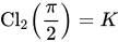
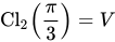
القيم الخاصة تذكر دالة بارنز G ، وثابت كاتالان K ، وثابت جيزيكينغ V. تتضمن بعض القيم الخاصة ما يلي:
Cl 2 ( π 2 ) = ك {\displaystyle \operatorname {Cl} _{2}\left({\frac {\pi }{2}}\right)=K} Cl 2 ( π 3 ) = V {\displaystyle \operatorname {Cl} _{2}\left({\frac {\pi }{3}}\right)=V} Cl 2 ( π 3 ) = 3 π سجل ( جي ( 2 3 ) جي ( 1 3 ) ) - 3 π سجل Γ ( 1 3 ) + π سجل ( 2 π 3 ) {\displaystyle \operatorname {Cl} _{2}\left({\frac {\pi }{3}}\right)=3\pi \log \left({\frac {G\left({\frac {2}{3}}\right)}{G\left({\frac {1}{3}}\right)}}\right)-3\pi \log \Gamma \left({\frac {1}{3}}\right)+\pi \log \left({\frac {2\pi }{\sqrt {3}}}\right)} Cl 2 ( 2 π 3 ) = 2 π سجل ( جي ( 2 3 ) جي ( 1 3 ) ) - 2 π سجل Γ ( 1 3 ) + 2 π 3 سجل ( 2 π 3 ) {\displaystyle \operatorname {Cl} _{2}\left({\frac {2\pi }{3}}\right)=2\pi \log \left({\frac {G\left({\frac {2}{3}}\right)}{G\left({\frac {1}{3}}\right)}}\right)-2\pi \log \Gamma \left({\frac {1}{3}}\right)+{\frac {2\pi }{3}}\log \left({\frac {2\pi }{\sqrt {3}}}\right)} Cl 2 ( π 4 ) = 2 π سجل ( جي ( 7 8 ) جي ( 1 8 ) ) - 2 π سجل Γ ( 1 8 ) + π 4 سجل ( 2 π 2 - 2 ) {\displaystyle \operatorname {Cl} _{2}\left({\frac {\pi }{4}}\right)=2\pi \log \left({\frac {G\left({\frac {7}{8}}\right)}{G\left({\frac {1}{8}}\right)}}\right)-2\pi \log \Gamma \left({\frac {1}{8}}\right)+{\frac {\pi }{4}}\log \left({\frac {2\pi }{\sqrt {2-{\sqrt {2}}}}}\right)} Cl 2 ( 3 π 4 ) = 2 π سجل ( جي ( 5 8 ) جي ( 3 8 ) ) - 2 π سجل Γ ( 3 8 ) + 3 π 4 سجل ( 2 π 2 + 2 ) {\displaystyle \operatorname {Cl} _{2}\left({\frac {3\pi }{4}}\right)=2\pi \log \left({\frac {G\left({\frac {5}{8}}\right)}{G\left({\frac {3}{8}}\right)}}\right)-2\pi \log \Gamma \left({\frac {3}{8}}\right)+{\frac {3\pi }{4}}\log \left({\frac {2\pi }{\sqrt {2+{\sqrt {2}}}}}\right)} Cl 2 ( π 6 ) = 2 π سجل ( جي ( 11 12 ) جي ( 1 12 ) ) - 2 π سجل Γ ( 1 12 ) + π 6 سجل ( 2 π 2 3 - 1 ) {\displaystyle \operatorname {Cl} _{2}\left({\frac {\pi }{6}}\right)=2\pi \log \left({\frac {G\left({\frac {11}{12}}\right)}{G\left({\frac {1}{12}}\right)}}\right)-2\pi \log \Gamma \left({\frac {1}{12}}\right)+{\frac {\pi }{6}}\log \left({\frac {2\pi {\sqrt {2}}}{{\sqrt {3}}-1}}\right)} Cl 2 ( 5 π 6 ) = 2 π سجل ( جي ( 7 12 ) جي ( 5 12 ) ) - 2 π سجل Γ ( 5 12 ) + 5 π 6 سجل ( 2 π 2 3 + 1 ) {\displaystyle \operatorname {Cl} _{2}\left({\frac {5\pi }{6}}\right)=2\pi \log \left({\frac {G\left({\frac {7}{12}}\right)}{G\left({\frac {5}{12}}\right)}}\right)-2\pi \log \Gamma \left({\frac {5}{12}}\right)+{\frac {5\pi }{6}}\log \left({\frac {2\pi {\sqrt {2}}}{{\sqrt {3}}+1}}\right)}
بشكل عام، من صيغة انعكاس دالة بارنز G ،
Cl 2 ( 2 π z ) = 2 π سجل ( جي ( 1 - z ) جي ( z ) ) - 2 π سجل Γ ( z ) + 2 π z سجل ( π الخطيئة π z ) {\displaystyle \operatorname {Cl} _{2}(2\pi z)=2\pi \log \left({\frac {G(1-z)}{G(z)}}\right)-2\pi \log \Gamma (z)+2\pi z\log \left({\frac {\pi }{\sin \pi z}}\right)}
وبصورة مكافئة، باستخدام صيغة أويلر للانعكاس لدالة غاما، إذن،
Cl 2 ( 2 π z ) = 2 π سجل ( جي ( 1 - z ) جي ( z ) ) - 2 π سجل Γ ( z ) + 2 π z سجل ( Γ ( z ) Γ ( 1 - z ) ) {\displaystyle \operatorname {Cl} _{2}(2\pi z)=2\pi \log \left({\frac {G(1-z)}{G(z)}}\right)-2\pi \log \Gamma (z)+2\pi z\log {\big (}\Gamma (z)\Gamma (1-z){\big )}}
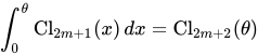
تكاملات الدالة المباشرة يمكن إثبات التكاملات التالية بسهولة من خلال تمثيلات المتسلسلة لدالة كلاوسن:
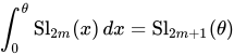
∫ 0 θ Cl 2 م ( x ) د x = ζ ( 2 م + 1 ) - Cl 2 م + 1 ( θ ) {\displaystyle \int _{0}^{\theta }\operatorname {Cl} _{2m}(x)\,dx=\zeta (2m+1)-\operatorname {Cl} _{2m+1}(\theta )} ∫ 0 θ Cl 2 م + 1 ( x ) د x = Cl 2 م + 2 ( θ ) {\displaystyle \int _{0}^{\theta }\operatorname {Cl} _{2m+1}(x)\,dx=\operatorname {Cl} _{2m+2}(\theta )} ∫ 0 θ سل 2 م ( x ) د x = سل 2 م + 1 ( θ ) {\displaystyle \int _{0}^{\theta }\operatorname {Sl} _{2m}(x)\,dx=\operatorname {Sl} _{2m+1}(\theta )} ∫ 0 θ سل 2 م + 1 ( x ) د x = ζ ( 2 م + 2 ) - سل 2 م + 2 ( θ ) {\displaystyle \int _{0}^{\theta }\operatorname {Sl} _{2m+1}(x)\,dx=\zeta (2m+2)-\operatorname {Sl} _{2m+2}(\theta )}
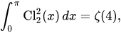
يمكن استخدام طرق التحليل الفورييه لإيجاد العزوم الأولى لمربع الدالةCl 2 ( x ) {\displaystyle \operatorname {Cl} _{2}(x)} [ 0 ، π ] {\displaystyle [0,\pi ]} [ 3 ]
∫ 0 π Cl 2 2 ( x ) د x = ζ ( 4 ) ، {\displaystyle \int _{0}^{\pi }\operatorname {Cl} _{2}^{2}(x)\,dx=\zeta (4),} ∫ 0 π ت Cl 2 2 ( x ) د x = 221 90720 π 6 - 4 ζ ( 5 ¯ ، 1 ) - 2 ζ ( 4 ¯ ، 2 ) ، {\displaystyle \int _{0}^{\pi }t\operatorname {Cl} _{2}^{2}(x)\,dx={\frac {221}{90720}}\pi ^{6}-4\zeta ({\overline {5}},1)-2\zeta ({\overline {4}},2),} ∫ 0 π ت 2 Cl 2 2 ( x ) د x = - 2 3 π [ 12 ζ ( 5 ¯ ، 1 ) + 6 ζ ( 4 ¯ ، 2 ) - 23 10080 π 6 ] . {\displaystyle \int _{0}^{\pi }t^{2}\operatorname {Cl} _{2}^{2}(x)\,dx=-{\frac {2}{3}}\pi \left[12\zeta ({\overline {5}},1)+6\zeta ({\overline {4}},2)-{\frac {23}{10080}}\pi ^{6}\right].}
هناζ {\displaystyle \zeta } دالة زيتا المتعددة .
التقييمات التكاملية التي تتضمن الدالة المباشرة يمكن حساب عدد كبير من التكاملات المثلثية واللوغاريتمية المثلثية باستخدام دالة كلاوسن، والعديد من الثوابت الرياضية الشائعة مثلك {\displaystyle \,K\,} ثابت كاتالان )،سجل 2 {\displaystyle \,\log 2\,} زيتا ،ζ ( 2 ) {\displaystyle \,\zeta (2)\,} ζ ( 3 ) {\displaystyle \,\zeta (3)\,}
الأمثلة المدرجة أدناه تتبع مباشرة من التمثيل التكاملي لدالة كلاوسن، ولا تتطلب البراهين أكثر من حساب المثلثات الأساسي والتكامل بالتجزئة والتكامل العرضي حدًا بحد لتعريفات متسلسلة فورييه لدوال كلاوسن.
∫ 0 θ سجل ( الخطيئة x ) د x = - 1 2 Cl 2 ( 2 θ ) - θ سجل 2 {\displaystyle \int _{0}^{\theta }\log(\sin x)\,dx=-{\tfrac {1}{2}}\operatorname {Cl} _{2}(2\theta )-\theta \log 2} ∫ 0 θ سجل ( كوس x ) د x = 1 2 Cl 2 ( π - 2 θ ) - θ سجل 2 {\displaystyle \int _{0}^{\theta }\log(\cos x)\,dx={\tfrac {1}{2}}\operatorname {Cl} _{2}(\pi -2\theta )-\theta \log 2} ∫ 0 θ سجل ( لون برونزي x ) د x = - 1 2 Cl 2 ( 2 θ ) - 1 2 Cl 2 ( π - 2 θ ) {\displaystyle \int _{0}^{\theta }\log(\tan x)\,dx=-{\tfrac {1}{2}}\operatorname {Cl} _{2}(2\theta )-{\tfrac {1}{2}}\operatorname {Cl} _{2}(\pi -2\theta )} ∫ 0 θ سجل ( 1 + كوس x ) د x = 2 Cl 2 ( π - θ ) - θ سجل 2 {\displaystyle \int _{0}^{\theta }\log(1+\cos x)\,dx=2\operatorname {Cl} _{2}(\pi -\theta )-\theta \log 2} ∫ 0 θ سجل ( 1 - كوس x ) د x = - 2 Cl 2 ( θ ) - θ سجل 2 {\displaystyle \int _{0}^{\theta }\log(1-\cos x)\,dx=-2\operatorname {Cl} _{2}(\theta )-\theta \log 2} ∫ 0 θ سجل ( 1 + الخطيئة x ) د x = 2 ك - 2 Cl 2 ( π 2 + θ ) - θ سجل 2 {\displaystyle \int _{0}^{\theta }\log(1+\sin x)\,dx=2K-2\operatorname {Cl} _{2}\left({\frac {\pi }{2}}+\theta \right)-\theta \log 2} ∫ 0 θ سجل ( 1 - الخطيئة x ) د x = - 2 ك + 2 Cl 2 ( π 2 - θ ) - θ سجل 2 {\displaystyle \int _{0}^{\theta }\log(1-\sin x)\,dx=-2K+2\operatorname {Cl} _{2}\left({\frac {\pi }{2}}-\theta \right)-\theta \log 2}
التصنيفات المخفية:
مقالات ذات وصف موجز الوصف المختصر يختلف عن ويكي بيانات جميع المقالات التي تحتوي على عبارات غير موثقة المصدر مقالات تتضمن تصريحات غير موثقة المصدر من يوليو 2013 






![{\displaystyle \theta ={\frac {\pi }{3}}+2m\pi \quad [m\in \mathbb {Z} ]}](https://wikimedia.org/api/rest_v1/media/math/render/svg/301caa56535304b0db827b753a2cd412f5665c12)

![{\displaystyle \theta =-{\frac {\pi }{3}}+2m\pi \quad [m\in \mathbb {Z} ]}](https://wikimedia.org/api/rest_v1/media/math/render/svg/2fae98e863733e316c672bdd9098be49e228b375)

















![{\displaystyle \,[0,\theta ].\,}](https://wikimedia.org/api/rest_v1/media/math/render/svg/0c44a38c13c401abf6dbb2f057fd64ed963a251d)





![{\displaystyle \operatorname {Cl} _{m+1}(2\theta )=2^{m}\left[\operatorname {Cl} _{m+1}(\theta )+(-1)^{m}\operatorname {Cl} _{m+1}(\pi -\theta )\right]}](https://wikimedia.org/api/rest_v1/media/math/render/svg/2441146c5765f07b3d22ff7d8ff9d94aa675b079)

![{\displaystyle \operatorname {Cl} _{2m}\left({\frac {\pi }{2}}\right)=2^{2m-1}\left[\operatorname {Cl} _{2m}\left({\frac {\pi }{4}}\right)-\operatorname {Cl} _{2m}\left({\frac {3\pi }{4}}\right)\right]=\beta (2m)}](https://wikimedia.org/api/rest_v1/media/math/render/svg/9ddd71810db9ae56ce6285cb7936562583ce2fba)










![{\displaystyle {\frac {d}{d\theta }}\operatorname {Cl} _{2}(\theta )={\frac {d}{d\theta }}\left[-\int _{0}^{\theta }\log \left|2\sin {\frac {x}{2}}\right|\,dx\,\right]=-\log \left|2\sin {\frac {\theta }{2}}\right|=\operatorname {Cl} _{1}(\theta )}](https://wikimedia.org/api/rest_v1/media/math/render/svg/4d9fa3c1d1d4975c26733d0592edcd47e0804bf8)







![\begin{aligned}\begin{aligned}\theta \log \tan \theta -\frac {1}{2}\int _{0}^{2\theta }\log \left(\tan {\frac {x}{2}}\right)\,dx\\[6pt]=\begin{aligned}\theta \log \tan \theta -\frac {1}{2}\int _{0}^{2\theta }\log \left(\frac {\sin(x/2)}{\cos(x/2)}}\right)\,dx\\[6pt]=\begin{aligned}\theta \log \tan \theta -\frac {1}{2}\int _{0}^{2\theta }\log \left(\frac {1}{2}}\right)\,dx {2\sin(x/2)}{2\cos(x/2)}}\right)\,dx\\[6pt]={}&\theta \log \tan \theta -{\frac {1}{2}}\int _{0}^{2\theta }\log \left(2\sin {\frac {x}{2}}\right)\,dx+{\frac {1}{2}}\int _{0}^{2\theta }\log \left(2\cos {\frac {x}{2}}\right)\,dx\\[6pt]={}&\theta \log \tan \theta +{\frac {1}{2}}\operatorname {Cl} _{2}(2\theta )+{\frac {1}{2}}\int _{0}^{2\theta }\log \left(2\cos {\frac {x}{2}}\right)\,dx.\end{aligned}}}](https://wikimedia.org/api/rest_v1/media/math/render/svg/ac1e40c055b307b1f1196786837809a1285052fb)












![{\displaystyle \operatorname {Cl} _{2m}\left({\frac {q\pi }{p}}\right)={\frac {1}{(2p)^{2m}(2m-1)!}}\,\sum _{j=1}^{p}\sin \left({\tfrac {qj\pi }{p}}\right)\,\left[\psi _{2m-1}\left({\tfrac {j}{2p}}\right)+(-1)^{q}\psi _{2m-1}\left({\tfrac {j+p}{2p}}\right)\right].}](https://wikimedia.org/api/rest_v1/media/math/render/svg/d0df3f90937e191358fb288f9f467cc4ac557350)
![{\displaystyle \operatorname {Cl} _{2m}\left({\frac {q\pi }{p}}\right)={\frac {1}{(2p)^{2m}}}\,\sum _{j=1}^{p}\sin \left({\tfrac {qj\pi }{p}}\right)\,\left[\zeta \left(2m,{\tfrac {j}{2p}}\right)+(-1)^{q}\zeta \left(2m,{\tfrac {j+p}{2p}}\right)\right].}](https://wikimedia.org/api/rest_v1/media/math/render/svg/60025ebbc6e7a7d1676a7fdf206d7a31a4348af4)




![{\displaystyle {\begin{aligned}&\operatorname {Cl} _{2m}\left({\frac {q\pi }{p}}\right)\\={}&\sum _{k=0}^{\infty }{\frac {\sin \left[(kp+1){\frac {q\pi }{p}}\right]}{(kp+1)^{2m}}}+\sum _{k=0}^{\infty }{\frac {\sin \left[(kp+2){\frac {q\pi }{p}}\right]}{(kp+2)^{2m}}}+\sum _{k=0}^{\infty }{\frac {\sin \left[(kp+3){\frac {q\pi \begin{aligned}} \right} \text{\sum_{k=0}^{\infty} \text{\sin \left[(kp+p-2)\frac {q\pi }{p}\right]}{(kp+p-2)^{2m}} \text{\sum_{k=0}^{\infty} \text{\sin \left[(kp+p-1)\frac {q\pi }{p}\right]}{(kp+p-1)^{2m}} \text{\sum_{k=0}^{\infty} \text{\sin \left[(kp+p)\frac {q\pi }{p}\right]}{(kp+p)^{2m}} \end{aligned ...](https://wikimedia.org/api/rest_v1/media/math/render/svg/0abb29e3b9265e66eb7018f652f04098a17d91d4)
![{\displaystyle {\begin{aligned}&\operatorname {Cl} _{2m}\left({\frac {q\pi }{p}}\right)=\sum _{j=1}^{p}\left\{\sum _{k=0}^{\infty }{\frac {\sin \left[(kp+j){\frac {q\pi {p}}\right]}{(kp+j)^{2m}}}\right\}\\={}&\sum _{j=1}^{p}{\frac {1}{p^{2m}}}\left\{\sum _{k=0}^{\infty }{\frac {\sin \left[(kp+j){\frac {q\pi {p}}\يمين]}{(k+(j/p))^{2m}}}\right\}\end{محاذاة}}}](https://wikimedia.org/api/rest_v1/media/math/render/svg/93d3a4f119b0cbb92e6147b61bd28451604b8ee8)



![{\displaystyle \sin \left[(kp+j){\frac {q\pi }{p}}\right]=(-1)^{kq}\sin {\frac {qj\pi }{p}}}](https://wikimedia.org/api/rest_v1/media/math/render/svg/1506219055a797a00176b8c46dd48bfafd65ff31)

![{\displaystyle {\begin{aligned}&\sum _{k=0}^{\infty }{\frac {(-1)^{kq}}{(k+(j/p))^{2m}}}=\sum _{k=0}^{\infty }{\frac {(-1)^{(2k)q}}{((2k)+(j/p))^{2m}}}+\sum _ {k=0}^{\infty }{\frac {(-1)^{(2k+1)q}}{((2k+1)+(j/p))^{2m}}}\\={}&\sum _{k=0}^{\infty }{\frac {1}{(2k+(j/p))^{2m}}}+(-1)^{q}\,\sum _{ك=0}^{\infty }{\frac {1}{(2k+1+(j/p))^{2m}}}\\={}&{\frac {1}{2^{p}}}\left[\sum _{k=0}^{\infty }{\frac {1}{(k+(j/2p))^{2m}}}+(-1)^{q}\,\sum _{k=0}^{\infty }{\frac {1}{(k+\left({\frac {j+p}{2p}}\right))^{2m}}}\right]\end{aligned}}}](https://wikimedia.org/api/rest_v1/media/math/render/svg/01ce051d7cfe0c8342394d252d02154385293cda)

![{\displaystyle {\frac {1}{2^{2m}(2m-1)!}}\left[\psi _{2m-1}\left({\tfrac {j}{2p}}\right)+(-1)^{q}\psi _{2m-1}\left({\tfrac {j+p}{2p}}\right)\right]}](https://wikimedia.org/api/rest_v1/media/math/render/svg/26128b06fdb94c2a6db03c6dadef51a6ba4f2418)
![{\displaystyle \operatorname {Cl} _{2m}\left({\frac {q\pi }{p}}\right)={\frac {1}{(2p)^{2m}(2m-1)!}}\,\sum _{j=1}^{p}\sin \left({\tfrac {qj\pi }{p}}\right)\,\left[\psi _{2m-1}\left({\tfrac {j}{2p}}\right)+(-1)^{q}\psi _{2m-1}\left({\tfrac {j+p}{2p}}\right)\right]}](https://wikimedia.org/api/rest_v1/media/math/render/svg/db9811ae712344b8f051869b880fd4c33014a83d)








![{\displaystyle {\frac {\operatorname {Cl} _{2}(\theta )}{\theta }}=3-\log \left[|\theta |\left(1-{\frac {\theta ^{2}}{4\pi ^{2}}}\right)\right]-{\frac {2\pi }{\theta }}\log \left({\frac {2\pi +\theta }{2\pi -\theta }}\right)+\sum _{n=1}^{\infty }{\frac {\zeta (2n)-1}{n(2n+1)}}\left({\frac {\theta }{2\pi }}\right)^{2n}.}](https://wikimedia.org/api/rest_v1/media/math/render/svg/3a1d4a1a5b2d04b3fd5d444f6f4ba039b7177983)
















![{\displaystyle [0,\pi ]}](https://wikimedia.org/api/rest_v1/media/math/render/svg/3e2a912eda6ef1afe46a81b518fe9da64a832751)

![{\displaystyle \int _{0}^{\pi }t^{2}\operatorname {Cl} _{2}^{2}(x)\,dx=-{\frac {2}{3}}\pi \left[12\zeta ({\overline {5}},1)+6\zeta ({\overline {4}},2)-{\frac {23}{10080}}\pi ^{6}\right].}](https://wikimedia.org/api/rest_v1/media/math/render/svg/d13a18ca3ea120e1cd61af71afab0eb1d9f6f29f)







