
Hyperbolic functions

In mathematics, hyperbolic functions are analogues of the ordinary trigonometric functions, but defined using the hyperbola rather than the circle. Just as the points (cos t, sin t) form a circle with a unit radius, the points (cosh t, sinh t) form the right half of the unit hyperbola. Also, similarly to how the derivatives of sin(t) and cos(t) are cos(t) and –sin(t), the derivatives of sinh(t) and cosh(t) are cosh(t) and sinh(t).
Hyperbolic functions are used to express the angle of parallelism in hyperbolic geometry. They are used to express Lorentz boosts as hyperbolic rotations in special relativity. They also occur in the solutions of many linear differential equations (such as the equation defining a catenary), cubic equations, and Laplace's equation in Cartesian coordinates. Laplace's equations are important in many areas of physics, including electromagnetic theory, heat transfer, and fluid dynamics.
The basic hyperbolic functions are:[1]
from which are derived:[4]
- الظل الزائدي " تانه " ( / ˈtæŋ , ˈtæntʃ , ˈθæn / ) ، [ 5 ]
- الظل الزائدي " coth " ( / ˈ k ɒ θ , ˈ k oʊ θ / ), [ 6 ] [ 7 ]
- القاطع الزائدي " sech " ( / ˈ s ɛ tʃ , ˈ ʃ ɛ k / ) ، [ 8 ]
- قاطع التمام الزائدي " csch " أو " cosech " ( / ˈkoʊsɛtʃ , ˈkoʊʃɛk / [ 3 ] )
بما يتوافق مع الدوال المثلثية المشتقة.
الدوال الزائدية العكسية هي:
- الجيب الزائدي العكسي " arsinh " (يرمز له أيضًا بـ " sinh −1 " أو " asinh " أو أحيانًا " arcsinh ") [ 9 ] [ 10 ] [ 11 ]
- دالة جيب التمام الزائدية العكسية " arcosh " (يشار إليها أيضًا باسم " cosh −1 " أو " acosh " أو أحيانًا " arccosh ").
- الظل الزائدي العكسي " artanh " (يُشار إليه أيضًا بـ " tanh −1 " أو " atanh " أو أحيانًا " arctanh ")
- دالة الظل الزائدي العكسي " arcoth " (يشار إليها أيضًا باسم " coth −1 " أو " acoth " أو أحيانًا " arccoth ")
- القاطع الزائدي العكسي " arsech " (يُشار إليه أيضًا بـ " sech −1 " أو " asech " أو أحيانًا " arcsech ")
- inverse hyperbolic cosecant "arcsch" (also denoted "arcosech", "csch−1", "cosech−1","acsch", "acosech", or sometimes "arccsch" or "arccosech")
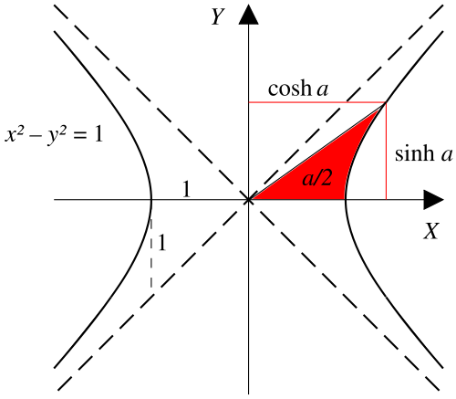
The hyperbolic functions take an argument called a hyperbolic angle. The magnitude of a hyperbolic angle is the area of its hyperbolic sector to xy = 1. The hyperbolic functions may be defined in terms of the legs of a right triangle covering this sector.
In complex analysis, the hyperbolic functions arise when applying the ordinary sine and cosine functions to an imaginary angle. The hyperbolic sine and the hyperbolic cosine are entire functions. As a result, the other hyperbolic functions are meromorphic in the whole complex plane.
By Lindemann–Weierstrass theorem, the hyperbolic functions have a transcendental value for every non-zero algebraic value of the argument.[12]
History
The first known calculation of a hyperbolic trigonometry problem is attributed to Gerardus Mercator when issuing the Mercator map projection circa 1566. It requires tabulating solutions to a transcendental equation involving hyperbolic functions.[13]
The first to suggest a similarity between the sector of the circle and that of the hyperbola was Isaac Newton in his 1687 Principia Mathematica.[14]
Roger Cotes suggested to modify the trigonometric functions using the imaginary unit to obtain an oblate spheroid from a prolate one.[14]

Hyperbolic functions were formally introduced in 1757 by Vincenzo Riccati.[14][13][15] Riccati used Sc. and Cc. (sinus/cosinus circulare) to refer to circular functions and Sh. and Ch. (sinus/cosinus hyperbolico) to refer to hyperbolic functions.[14] As early as 1759, Daviet de Foncenex showed the interchangeability of the trigonometric and hyperbolic functions using the imaginary unit and extended de Moivre's formula to hyperbolic functions.[15][14]
During the 1760s, Johann Heinrich Lambert systematized the use functions and provided exponential expressions in various publications.[14][15] Lambert credited Riccati for the terminology and names of the functions, but altered the abbreviations to those used today.[15][16]
Notation
Definitions
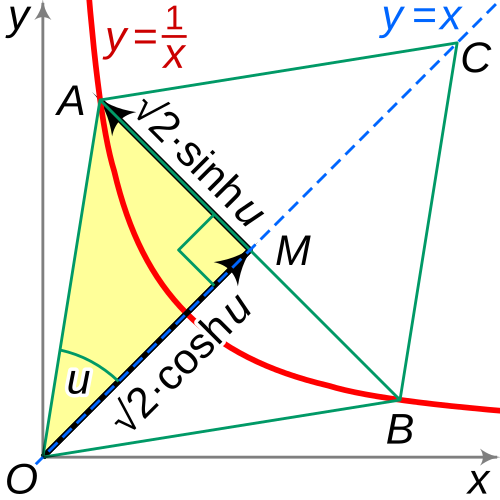
With hyperbolic angleu, the hyperbolic functions sinh and cosh can be defined with the exponential function eu.[1][4] In the figure .

Exponential definitions
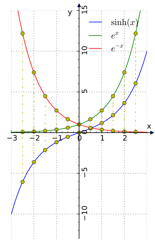
- Hyperbolic sine: the odd part of the exponential function, that is,
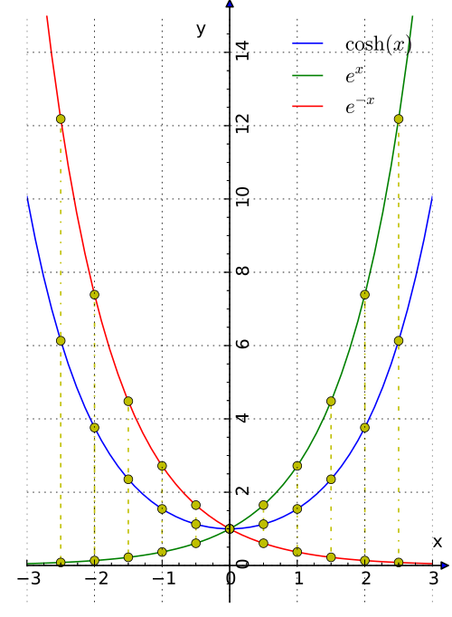
- Hyperbolic cosine: the even part of the exponential function, that is,


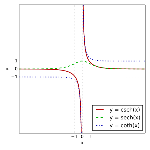
- Hyperbolic tangent:
- Hyperbolic cotangent: for x ≠ 0,
- Hyperbolic secant:
- Hyperbolic cosecant: for x ≠ 0,




Differential equation definitions
The hyperbolic functions may be defined as solutions of differential equations: The hyperbolic sine and cosine are the solution (s, c) of the system with the initial conditions The initial conditions make the solution unique; without them any pair of functions would be a solution.
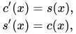


sinh(x) and cosh(x) are also the unique solution of the equation f″(x) = f(x), such that f(0) = 1, f′(0) = 0 for the hyperbolic cosine, and f(0) = 0, f′(0) = 1 for the hyperbolic sine.
Complex trigonometric definitions
Hyperbolic functions may also be deduced from trigonometric functions with complex arguments:
- Hyperbolic sine:[1]
- Hyperbolic cosine:[1]
- Hyperbolic tangent:
- Hyperbolic cotangent:
- Hyperbolic secant:
- Hyperbolic cosecant:






where i is the imaginary unit with i2 = −1.
The above definitions are related to the exponential definitions via Euler's formula (See § Hyperbolic functions for complex numbers below).
Characterizing properties
Hyperbolic cosine
It can be shown that the area under the curve of the hyperbolic cosine (over a finite interval) is always equal to the arc length corresponding to that interval:[17]

Hyperbolic tangent
The hyperbolic tangent is the (unique) solution to the differential equationf′ = 1 − f2, with f(0) = 0.[18][19]
Useful relations
The hyperbolic functions satisfy many identities, all of them similar in form to the trigonometric identities. In fact, Osborn's rule[20] (named after George Osborn) states that one can convert any trigonometric identity (up to but not including sinhs or implied sinhs of 4th degree) for , , or and into a hyperbolic identity, by:


- expanding it completely in terms of integral powers of sines and cosines,
- changing sine to sinh and cosine to cosh, and
- switching the sign of every term containing a product of two sinhs.
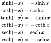
Reciprocals:
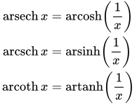
Analogous to Euler's formula:
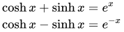
Analogous to the Pythagorean trigonometric identity:

Sums and differences of arguments
خصوصًا

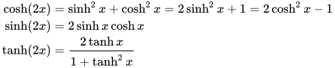
صيغ الجمع والطرح

تركيبات المنتجات
![\begin{aligned}\cosh x\,\cosh y&={\tfrac {1}{2}}{\bigl (}\!\!~\cosh(x+y)+\cosh(xy){\bigr )}\\[5mu]\sinh x\,\sinh y&={\tfrac {1}{2}}{\bigl (}\!\!~\cosh(x+y)-\cosh(xy){\bigr )}\\[5mu]\sinh x\,\cosh y&={\tfrac {1}{2}}{\bigl (}\!\!~\sinh(x+y)+\sinh(xy){\bigr )}\\[5mu]\cosh x\,\sinh y&={\tfrac {1}{2}}{\bigl (}\!\!~\sinh(x+y)-\sinh(xy){\bigr )}\\[5mu]\end{aligned}}}](https://wikimedia.org/api/rest_v1/media/math/render/svg/ebcc6e905df736163061cf56b304ab50d7853739)
صيغ نصف الوسيط
![\begin{aligned}\sinh \left(\frac {x}{2}\right)&=\frac {\sinh x}{\sqrt {2(\cosh x+1)}}}&&=\operatorname {sgn} x\,{\sqrt {\frac {\cosh x-1}{2}}}\\[6px]\cosh \left(\frac {x}{2}}\right)&=\sqrt {\frac {\cosh x+1}{2}}}\\[6px]\tanh \left(\frac {x}{2}}\right)&=\frac {\sinh x}{\cosh x+1}}&&=\operatorname {sgn} x\,{\sqrt {\frac {\cosh x-1}{\cosh x+1}}}=\frac {e^{x}-1}{e^{x}+1}}\end{aligned}}}](https://wikimedia.org/api/rest_v1/media/math/render/svg/412a4ffd109486f684e515634b33447b13444954)
حيث sgn هي دالة الإشارة .
إذا كان x ≠ 0 فإن

صيغ نصف وسيط الظل
عندما،


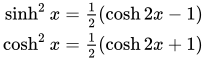
الصيغ المربعة
عدم المساواة
المتباينة التالية مفيدة في الإحصاء: [ 21 ]

ويمكن إثبات ذلك من خلال مقارنة متسلسلة تايلور للدالتين حدًا بحد.
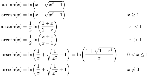
الدوال العكسية كلوغاريتمات
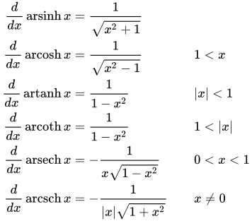
المشتقات

المشتقات الثانية
كل من الدالتين sinh و cosh تساوي مشتقتها الثانية ، أي:
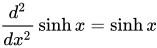
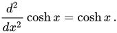
جميع الدوال التي تتمتع بهذه الخاصية هي تركيبات خطية من دالتي sinh و cosh ، وخاصة الدوال الأسية.و[ 22 ]


التكاملات القياسية
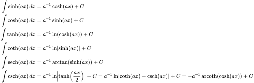
يمكن إثبات التكاملات التالية باستخدام التعويض الزائدي :
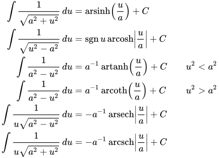
حيث C هو ثابت التكامل .
تعبيرات متسلسلة تايلور
من الممكن التعبير بشكل صريح عن متسلسلة تايلور عند الصفر (أو متسلسلة لوران ، إذا لم تكن الدالة معرفة عند الصفر) للدوال المذكورة أعلاه.
هذه المتسلسلة متقاربة لكل قيمة عقدية لـ x . وبما أن دالة sinh x فردية ، فإن الأسس الفردية فقط لـ x تظهر في متسلسلة تايلور الخاصة بها.

هذه المتسلسلة متقاربة لكل قيمة عقدية لـ x . وبما أن الدالة cosh x زوجية ، فإن الأسس الزوجية فقط لـ x تظهر في متسلسلة تايلور الخاصة بها.

مجموع متسلسلتي sinh و cosh هو تعبير المتسلسلة اللانهائية للدالة الأسية .
تلي السلسلة التالية وصف لمجموعة فرعية من مجال تقاربها ، حيث تكون السلسلة متقاربة ومجموعها يساوي الدالة.
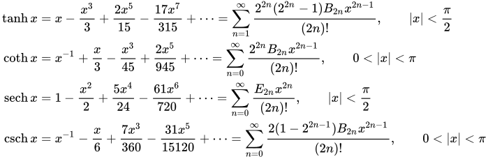
أين:


المنتجات اللانهائية والكسور المستمرة
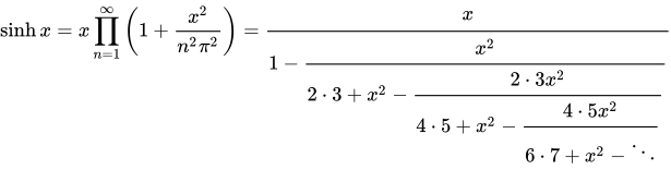
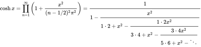
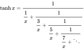
تكون التوسعات التالية صالحة في المستوى المركب بأكمله:
مقارنة بالدوال الدائرية
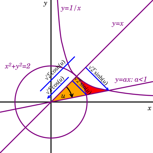
The hyperbolic functions represent an expansion of trigonometry beyond the circular functions. Both types depend on an argument, either circular angle or hyperbolic angle.
Since the area of a circular sector with radius r and angle u (in radians) is r2u/2, it will be equal to u when r = √2. In the diagram, such a circle is tangent to the hyperbola xy = 1 at (1, 1). The yellow sector depicts an area and angle magnitude. Similarly, the yellow and red regions together depict a hyperbolic sector with area corresponding to hyperbolic angle magnitude.
The legs of the two right triangles with the hypotenuse on the ray defining the angles are of length √2 times the circular and hyperbolic functions.
The hyperbolic angle is an invariant measure with respect to the squeeze mapping, just as the circular angle is invariant under rotation.[23]
The Gudermannian function gives a direct relationship between the circular functions and the hyperbolic functions that does not involve complex numbers.
The graph of the function is the catenary, the curve formed by a uniform flexible chain, hanging freely between two fixed points under uniform gravity.

Relationship to the exponential function
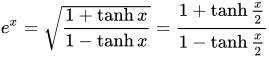
The decomposition of the exponential function in its even and odd parts gives the identities and Combined with Euler's formula this gives for the general complex exponential function.




Additionally,
Hyperbolic functions for complex numbers
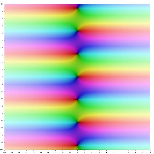 |  | 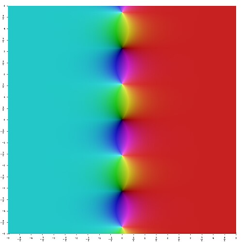 | 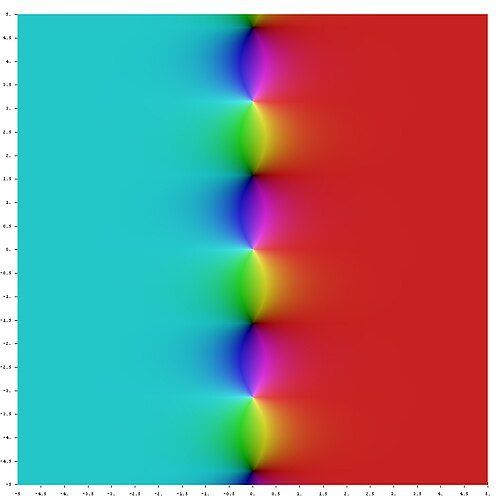 | 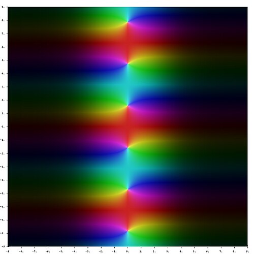 | 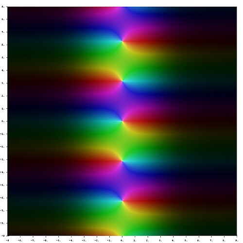 |


Since the exponential function can be defined for any complex argument, we can also extend the definitions of the hyperbolic functions to complex arguments. The functions sinh z and cosh z are then holomorphic.
تُعطى العلاقات مع الدوال المثلثية العادية بواسطة صيغة أويلر للأعداد المركبة: لذا:
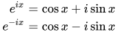

وبالتالي، فإن الدوال الزائدية دورية بالنسبة للمكون التخيلي، ولها دورة.((للدالة الظل الزائدي ودالة ظل التمام).


انظر أيضاً
مراجع
- 1 2 3 4 وايسشتاين، إريك دبليو. "الدوال الزائدية" . mathworld.wolfram.com . تم الاطلاع عليه بتاريخ 29-08-2020 .
- ↑ (1999) قاموس كولينز المختصر ، الطبعة الرابعة، هاربر كولينز، غلاسكو، رقم ISBN 0 00 472257 4، ص 1386
- 1 2 قاموس كولينز المختصر ، ص 328
- 1 2 "الدوال الزائدية" . www.mathsisfun.com . تم الاطلاع عليه بتاريخ 29-08-2020 .
- ↑ قاموس كولينز المختصر ، ص 1520
- ↑ قاموس كولينز المختصر ، ص 329
- ↑ tanh
- ↑ قاموس كولينز المختصر ، ص 1340
- ↑ وودهاوس، ن.م.ج. (2003)، النسبية الخاصة ، لندن: سبرينغر، ص 71، رقم ISBN 978-1-85233-426-0
- ↑ أبراموفيتز، ميلتون ؛ ستيجون، إيرين أ. ، محرران (1972)، دليل الدوال الرياضية مع الصيغ والرسوم البيانية والجداول الرياضية ، نيويورك: منشورات دوفر ، ISBN 978-0-486-61272-0
- ↑ بعض الأمثلة على استخدام دالة arcsinh الموجودة في كتب جوجل .
- ↑ نيفن، إيفان (1985). الأعداد غير النسبية . المجلد 11. الجمعية الرياضية الأمريكية. ISBN 9780883850381JSTOR 10.4169/ j.ctt5hh8zn .
- 1 2 جورج ف. بيكر؛ سي إي فان أورستراند (1909). الدوال الزائدية . المكتبة الرقمية العالمية. مؤسسة سميثسونيان.
- 1 2 3 4 5 6 ماكماهون، جيمس (1896). الدوال الزائدية . جامعة عثمانية، المكتبة الرقمية للهند. جون وايلي وأولاده.
- 1 2 3 4 برادلي، روبرت إي.؛ دانتونيو، لورانس أ.؛ سانديفير، تشارلز إدوارد. أويلر في عام 300: تقدير. الجمعية الرياضية الأمريكية، 2007. صفحة 100.
- ↑Becker, Georg F. Hyperbolic functions. Read Books, 1931. Page xlviii.
- ↑N.P., Bali (2005). Golden Integral Calculus. Firewall Media. p. 472. ISBN 81-7008-169-6.
- ↑Steeb, Willi-Hans (2005). Nonlinear Workbook, The: Chaos, Fractals, Cellular Automata, Neural Networks, Genetic Algorithms, Gene Expression Programming, Support Vector Machine, Wavelets, Hidden Markov Models, Fuzzy Logic With C++, Java And Symbolicc++ Programs (3rd ed.). World Scientific Publishing Company. p. 281. ISBN 978-981-310-648-2.Extract of page 281 (using lambda=1)
- ↑Oldham, Keith B.; Myland, Jan; Spanier, Jerome (2010). An Atlas of Functions: with Equator, the Atlas Function Calculator (2nd, illustrated ed.). Springer Science & Business Media. p. 290. ISBN 978-0-387-48807-3.Extract of page 290
- ↑Osborn, G. (July 1902). "Mnemonic for hyperbolic formulae". The Mathematical Gazette. 2 (34): 189. doi:10.2307/3602492. JSTOR 3602492. S2CID 125866575.
- ↑Audibert, Jean-Yves (2009). "Fast learning rates in statistical inference through aggregation". The Annals of Statistics. p. 1627.
- ↑Olver, Frank W. J.; Lozier, Daniel M.; Boisvert, Ronald F.; Clark, Charles W., eds. (2010), "Hyperbolic functions", NIST Handbook of Mathematical Functions, Cambridge University Press, ISBN 978-0-521-19225-5, MR 2723248.
- ↑Haskell, Mellen W., "On the introduction of the notion of hyperbolic functions", Bulletin of the American Mathematical Society1:6:155–9, full text
External links
- "Hyperbolic functions", Encyclopedia of Mathematics, EMS Press, 2001 [1994]
- Hyperbolic functions on PlanetMath
- GonioLab: Visualization of the unit circle, trigonometric and hyperbolic functions (Java Web Start)
- Web-based calculator of hyperbolic functions
- Hyperbolic functions
- Exponentials
- Hyperbolic geometry
- Analytic functions
- Sigmoid functions